Range minimum query
The term range minimum query (RMQ) comprises all variations of the problem of finding the smallest element (or the position of the smallest element) in a contiguous subsequence of a list of items taken from a totally ordered set (usually numbers). This is one of the most extensively-studied problems in computer science, and many algorithms are known, each of which is appropriate for a specific variation.
A single range minimum query is a set of indices  into an array
  ; the answer to this query is some
  (see half-open interval) such that
  for all
  . In isolation, this query is answered simply by scanning through the range given and selecting the minimum element, which can take up to linear time. The problem is interesting because we often desire to answer a large number of queries, so that if, for example, 500000 queries are to be performed on a single array of 10000000 elements, then using this naive approach on each query individually is probably too slow.
Contents
Static
In the static range minimum query, the input is an array and a set of intervals (contiguous subsequences) of the array, identified by their endpoints, and for each interval we must find the smallest element contained therein. Modifications to the array are not allowed, but we must be prepared to handle queries "on the fly"; that is, we might not know all of them at once.
Sliding
This problem can be solved in linear time in the special case in which the intervals are guaranteed to be given in such an order that they are successive elements of a sliding window; that is, each interval given in input neither starts earlier nor ends later than the previous one. This is the sliding range minimum query problem; an algorithm is given in that article.
Naive precomputation
This approach involves precomputing the minimum of every possible range in the given array and storing all the results in a table; this table will use up  space but queries will be answerable in constant time. This table can also be computed in time by noting that the minimum of a range
  occurs either in the last element,
  , or in the rest of it,
  , so that given the minimum in range
  we can compute that of
  in constant time.
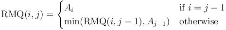
Formally, we use the recurrence
Division into blocks
In all other cases, we must consider other solutions. A simple solution for this and other related problems involves splitting the array into equally sized blocks (say,  elements each) and precomputing the minimum in each block. This precomputation will take
  time, since it takes
  time to find the minimum in each block, and there are
  blocks.
After this, when we are given some query  , we note that this can be written as the union of the intervals
  , where all the intervals except for the first and last are individual blocks. If we can find the minimum in each of these subintervals, the smallest of those values will be the minimum in . But because all the intervals in the middle (note that there may be zero of these if
  and
and  are in the same block) are blocks, their minima can simply be looked up in constant time.
Observe that the intermediate intervals are  in number (because there are only about
  blocks in total). Furthermore, if we pick
  at the nearest available block boundary, and likewise with
  , then the intervals
  and
and  have size
  (since they do not cross block boundaries). By taking the minimum of all the precomputed block minima, and the elements in and , the answer is obtained in
 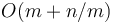 time. If we choose a block size of
  , we obtain
  overall.
Segment tree
While is not optimal, it is certainly better than linear time, and suggests that we might be able to do better using precomputation. Instead of dividing the array into  pieces, we might consider dividing it in half, and then dividing each half in half, and dividing each quarter in half, and so on. The resulting structure of intervals and subintervals is a segment tree. It uses linear space and requires linear time to construct; and once it has been built, any query can be answered in
  time.
time.
Sparse table
(Namely due to [1].) At the expense of space and preprocessing time, we can even answer queries in  using dynamic programming. Define
  to be the minimum of the elements
 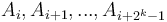 (or as many of those elements as actually exist); that is, the elements in an interval of size
  starting from
  . Then, we see that
  for each , and
 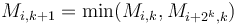 ; that is, the minimum in an interval of size
  is the smaller of the minima of the two halves of which it is composed, of size . Thus, each entry of
  can be computed in constant time, and in total has about
  entries (since values of
  for which
  are not useful). Then, given the query , simply find such that
  and
and  overlap but are contained within ; then we already know the minima in each of these two sub-intervals, and since they cover the query interval, the smaller of the two is the overall minimum. It's not too hard to see that the desired is
  ; and then the answer is
  .
.
Cartesian trees
We can get the best of both worlds—that is, constant query time and linear preprocessing time and space—but the algorithm is somewhat more involved. It combines the block-based approach, the sparse table approach, and the use of Cartesian trees.
We observe that some minimum in a range in the given array occurs at the same place as the lowest common ancestor of the two nodes corresponding to the endpoints of the range in the Cartesian tree of the array. That is, if elements  and
and  occur at nodes
  and
and  in the Cartesian tree of , then there is some
  in the range
  such that the element occurs at the lowest common ancestor of and in the Cartesian tree.
Proof: An inorder traversal of the Cartesian tree gives the original array. Thus, consider the segment  of the inorder traversal beginning when is visited and is visited ( and are as above); this must be equivalent to the segment of the array . Now, if the LCA of and is , then is in its right subtree; but must then contain only and elements from 's right subtree, since all nodes in 's right subtree (including ) will be visited immediately after itself; so that all nodes in are descendants of . Likewise, if is the LCA, then consists entirely of descendants of . If the LCA is neither nor , then must occur in its left subtree and in its right subtree (because if they both occurred in the same subtree, then the root of that subtree would be a lower common ancestor, a contradiction). But all elements in the left subtree of the LCA, including are visited immediately before the LCA, and all elements in the right, including , are visited immediately after the LCA, and hence, again, all nodes in are descendants of the LCA. Now, the labels on the nodes in correspond to the elements
  , and all nodes in have labels less than or equal to the label of the LCA, since Cartesian trees are min-heap-ordered; so it follows that the label of the LCA is the minimum element in the range.
Cartesian trees may be constructed in linear time and space, so we are within our  preprocessing bound so far; we just need to solve the LCA problem on the Cartesian tree. We will do this, curiously enough, by reducing it back to RMQ (with linear preprocessing time) using the technique described in the Lowest common ancestor article. However, the array derived from the LCA-to-RMQ reduction (which we'll call
  ) has the property that any two adjacent elements differ by +1 or -1. We now focus on how to solve this restricted form of RMQ with linear preprocessing time and constant query time.
First, divide into blocks of size roughly  . Find the minimum element in each block and construct an array
  such that
  is the minimum in the leftmost block,
  in the second-leftmost block, and so on. Construct a sparse table from array . Now, if we are given a range consisting of any number of consecutive blocks in , then the minimum of this range is given by the minimum of the corresponding minima in ---and, since we have constructed the sparse table of , this query can be answered in constant time. Array has size
  , so its sparse table is computed using time and space
  .
.
Now consider an individual block of . If we fix the first element of this block, then there are  possible combinations of values for the entire block, since with each following element we have a choice between two alternatives (it is either greater or less than the previous element by 1). Say that two blocks have the same kind if their corresponding elements differ by a constant (e.g., [2,1,2,3,4] and [0,-1,0,1,2] are of the same kind). Hence there are only different kinds of blocks; and, furthermore, all blocks of a given kind have their minimum in the same position, regardless of the actual values of the elements. Therefore, for each kind of block, we will naively precompute all possible range minimum queries for that block. But each block has size
  , so the precomputation uses
  space and time; and in total there are blocks, so in total this precomputation stage uses
  space and time. Finally, for each block in , compute its kind, and store the result in another auxiliary array
  . (This will use linear time and space.)
Now, we use the block-based approach to answering a query. We divide the interval given up into at most three subintervals. The first goes from the initial element to the last element of its block; the second spans zero or more complete blocks; and the third ends at the final element of the given interval and begins at the first element of its block. The minimum element is in one of these three subintervals. To find the minimum in the first subinterval, we look up the kind of block it is contained in (using array ), and then look up the precomputed position of the minimum in the desired range for that specific kind of block; and finally we look up the value at that position in . We do something similar for the third subinterval. For the second subinterval, we use the sparse table lookup discussed two paragraphs above. The query is answered in constant time overall.
Dynamic
The block-based solution handles the dynamic case as well; we must simply remember, whenever we update an element, to recompute the minimum element in the block it is in. This gives time per update, and, assuming a uniform random distribution of updates, the expected update time is . This is because if we decrease an element, we need only check whether the new value is less than the current minimum (constant time), whereas if we increase an element, we only need to recompute the minimum if the element updated was the minimum before (which takes time but has a probability of occurring of only  ). Unfortunately, the query still has average-case time .
The segment tree can be computed in linear time and allows both queries and updates to be answered in  time. It also allows, with some cleverness, entire ranges to be updated at once (efficiently). Analysis of the average case is left as an exercise to the reader.
We can also use any balanced binary tree (or dictionary data structure such as a skip-list) and augment it to support range minimum query operations with O(log n) per Update (Insert/Delete) as well as Query.
References
Much of the information in this article was drawn from a single source:
- ↑ "Range Minimum Query and Lowest Common Ancestor". (n.d.). Retrieved from http://community.topcoder.com/tc?module=Static&d1=tutorials&d2=lowestCommonAncestor#Range_Minimum_Query_%28RMQ%29