Dynamic programming
Dynamic programming (DP) is a technique for solving problems that involves computing the solution to a large problem using previously-computed solutions to smaller problems. DP, however, differs from recursion in that in DP, one solves the smallest possible subproblems (the base cases) first, and works up to the original problem, storing the solution to each subproblem in a table (usually a simple array or equivalent data structure) as it is computed so that its value can be quickly looked up when computing the solutions to larger subproblems. Most problems that are solved using DP are either counting problems or optimization problems, but there are others that fall into neither category. Because DP is a scheme for solving problems rather than a specific algorithm, its applicability is extremely broad, and so a number of examples are presented in this article to help explain exactly what DP is and what it can be used for.
By some estimates, nearly a third of all problems that appear on the IOI and national olympiads and team selection competitions are intended to be solved using DP. This may have decreased in modern years, since competitors are getting better and better at solving DP problems. (The high incidence of DP problems on the Canadian Computing Competition, for one, will become evident in the examples below.)
Contents
Basic principles of DP
Not every optimization problem can be solved using DP, just as not every optimization problem can be solved using recursion. In order for an optimization problem to be solvable using DP, it must have the property of optimal substructure. And most of the time, when DP is useful, the problem will exhibit overlapping subproblems. (We can solve problems using DP even when they do not exhibit overlapping subproblems; but such problems can also easily be solved using naive recursive methods.) We will examine the problem Plentiful Paths from the 1996 Woburn Challenge and show how it exhibits both properties.
Optimal substructure
An optimization problem is said to have optimal substructure when it can be broken down into subproblems and the optimal solution to the original problem can be computed from the optimal solutions of the subproblems. Another way of saying this is that the optimal solution to a large problem contains an optimal solution (sometimes more than one) for a subproblem (maybe more than one). This is often stated and proved in its contrapositive form, which is that if a solution to a problem instance contains any suboptimal solutions to subinstances, then the solution is not optimal for the original instance. Let's put this into the context of Plentiful Paths.
The Plentiful Paths problem asks us to optimize the number of apples collected in travelling from the lower-left square to the upper-right square. We start at (1,1) and end up eventually at (M,N). It is fairly clear that at some point we must pass through either (M-1,N) or (M,N-1). (Think about this carefully if you don't see why this is.) Suppose that the optimal solution involved travelling through (M-1,N). So we take some path to reach (M-1,N) and then we take one step to reach the end, (M,N). A bit of thought should convince you that we must collect as many apples as possible on the path from (1,1) to (M-1,N) if we want to collect the maximum possible number of apples on the path from (1,1) to (M,N). This is because if we found a better path to get to (M-1,N) - that is, one with more apples along the way - then we would also collect more apples in total getting to (M,N).
Having said that, the optimal path to (M-1,N) must itself consist of an optimal path to one of the squares immediately before it, for the same reason: either (M-2,N) or (M-1,N-1)... and so on.
(Notice that if A is a subproblem of B, and B is a subproblem of C, then A is a subproblem of C as well. Then, a DP solution would first solve A, then use this to solve B, and finally use that to solve C. But if A is a subproblem of B, B cannot be a subproblem of A. This is because, in order to find an optimal solution to B, we would first need an optimal solution to A, but to find an optimal solution to A, we would first need an optimal solution to B, so ultimately we can solve neither problem.)
The Plentiful Paths problem has optimal substructure because any optimal solution to an instance of Plentiful Paths contains an optimal solution to a subproblem. In general, in a DP solution, we start by solving the smallest possible subproblems (such as: "how many apples can we collect going from (1,1) to (1,1)?") and work our way up to larger problems.
Overlapping subproblems
A problem is said to have overlapping subproblems when some of its subproblems are repeated. For example, in Plentiful Paths, in order to find an optimal path to (M,N), we must find the optimal paths to (M-1,N) and (M,N-1). To find the optimal path to (M-1,N), we need to find the optimal paths to both (M-2,N) and (M-1,N-1); to find the optimal path to (M,N-1) we must find the optimal path to both (M-1,N-1) and (M,N-2). Notice that the subproblem (M-1,N-1) was repeated. It is the fact that subproblems are repeated that gives DP its massive efficiency advantage over the recursive solution in the next section.
Example: recursive solution to Plentiful Paths
Based on the optimal substructure property of the Plentiful Paths problem, we might write the following pseudocode:
function plentiful_paths(A,x,y)
     if x=1
          if y=1 then
               return A[x,y]
          else
               return A[x,y]+plentiful_paths(A,x,y-1)
     else
          if y=1 then
               return A[x,y]+plentiful_paths(A,x-1,y)
          else
               return A[x,y]+max(plentiful_paths(A,x-1,y),plentiful_paths(A,x,y-1))
input M,N,A
print plentiful_paths(A,M,N)
Here, A is a matrix (two-dimensional array) in which an entry is 1 if the corresponding position in the grid contains an apple and 0 if it does not contain an apple; the function plentiful_paths(A,x,y) returns the maximum number of apples that can be retrieved in going from (1,1) to (x,y) in grid A.
- If x and y are both 1, then the question is how many apples we can collect if we travel from (1,1) to (1,1); this will simply be 1 if there is an apple at (1,1) and 0 otherwise. (That is the quantity A[x,y].)
- If x is 1 but y is not, then in order to travel from (1,1) to (x,y), we must first travel from (1,1) to (x,y-1), then take one step to reach (x,y). The maximum number of apples we can collect in travelling to (x,y) is equal to the maximum number of apples we can collect in travelling to (x,y-1) (this is plentiful_paths(A,x,y-1)), plus one if there is an apple at (x,y).
- Similarly, if x is not 1 and y is 1, then we collect the maximum number of apples in travelling to (x-1,y), then we add one apple if there is an apple in the square (x,y).
If x and y are both greater than 1, then the optimal path to (x,y) goes through either (x-1,y) or (x,y-1). The maximum number of apples collected in reaching (x,y) will be either the maximum number of apples collected in reaching (x-1,y) or the same for (x,y-1), whichever is greater (that is to say, max(plentiful_paths(A,x-1,y),plentiful_paths(A,x,y-1))), plus one if there is an apple at (x,y).
The problem with this recursive solution is that, even though the value of plentiful_paths(A,i,j) will be the same every time it is calculated as long as A, i, and j stay the same, it might calculate that value hundreds of times. For example, in calculating plentiful_paths(A,5,5), we will actually calculate plentiful_paths(A,1,1) seventy times. This is because of the overlapping subproblems. For larger grids, we waste so much time recalculating values that the algorithm becomes impractically slow and therefore unusable. We can avoid this by using memoization. However, DP presents an alternative solution.
(Note that in a real recursive solution we would not pass A by value, since its value never changes and thus passing by value would slow down the solution massively by copying A over and over again. Instead, A would be either passed by reference or stored as a global variable. In the latter case, it would disappear from the parameter list altogether.)
Example: dynamic solution to Plentiful Paths
input M,N,A
for x = 1 to M
     for y = 1 to N
          if x=1 then
               if y=1 then
                    dp[x,y]=A[x,y]
               else
                    dp[x,y]=A[x,y]+dp[x,y-1]
          else
               if y=1 then
                    dp[x,y]=A[x,y]+dp[x-1,y]
               else
                    dp[x,y]=A[x,y]+max(dp[x-1,y],dp[x,y-1])
print dp[M,N]
In the dynamic solution, dp[x,y] represents the maximum possible number of apples that can be obtained on some path from (1,1) to (x,y). As soon as we calculate this value, we store it in the two-dimensional array dp[]. We see that this solution follows essentially the same logic as the recursive solution, and our final answer is dp[M,N]. However, no entry in the dp[] table is calculated more than once. When M and N are each 1000, it would take far longer than the age of the universe for the recursive solution to finish executing even if the entire surface of the Earth were covered in transistors being used exclusively to execute the algorithm, but the dynamic solution would run in under a second on a modern desktop computer.
This solution exemplifies both the optimal substructure property (because in calculating dp[x,y], an optimal solution for the square (x,y) we potentially examine the values of dp[x-1,y] and dp[x,y-1], optimal solutions for possible preceding squares, or subproblems) and the overlapping subproblems property (most entries in the dp[] table will be examined twice, but only calculated once). It is the presence of overlapping subproblems that gives DP such a huge efficiency advantage over the naive recursive solution: we will only calculate the solution to each subproblem once, and from then on we will look it up whenever it is needed. Finally, we have computed the solution bottom-up, by solving the smallest subproblems first so that by the time we reach a particular subproblem, we have already computed the solutions to any subproblems on which that subproblem depends. Contrast this with the recursive solution, which considers the largest subproblem (the original problem) first; it is top-down.
Optimization example: Change problem
Dynamic change is the name given to a well-known algorithm for determining how to make change for a given amount of money using the fewest possible coins, assuming that we have an unlimited supply of coins of every denomination. For example, if the available denominations are 1 cent, 5 cents, 10 cents, and 25 cents, then we can make change for 48 cents by using one 25-cent coin, one 10-cent coins, two 5-cent,and three 1-cent coins, that is, 7 coins in total. There are other ways to make change for the same amount (for example, four 10-cent coins and eight 1-cent coins), but they all use 12 coins. Other sets of denominations are not so easy; for example, suppose we have at our disposal 17-cent, 14-cent, 9-cent, and 7-cent coins. It is now not immediately obvious how best to make change for a dollar (The solution is to use four 17-cent coins, one 14-cent coin, and two 9-cent coins.) Nor is it immediately obvious that it is impossible to make change for 29 cents.
The problem Golf from the 2000 Canadian Computing Competition is exactly analogous. Here, the distance to the hole is the amount for which we wish to make change, and each golf club is a denomination with value equal to how far it will hit the golf ball.
The general form of this problem is: given  , find
  such that
  and
and  is minimal.
  corresponds to the amount we wish to change, each
  to a denomination, and each
  to the number of coins of a given denomination we wish to use.
This problem exhibits optimal substructure in the following sense. Suppose we have found out how to make change for cents using some minimal collection of coins, and we take one coin away (with value  ), leaving a collection of coins with total value
  . Then, what we are left with must be an optimal way to make change for . This is because if we had any better way (fewer coins) of making change for , then we could just add the coin of value back in, and get a better way of making change for cents than what we originally assumed was minimal, a contradiction.
For example, if we have 48 cents in the form of one 25-cent coin, one 10-cent coins, two 5-cent coins, and three 1-cent coins, and we take away the 25-cent coin, then we are left with one 10-cent coins, two 5-cent coins, and three 1-cent coins, that is, 6 coins totalling 23 cents. However, 7 coins is not the least number of coins required to change 23 cents; we could do it in 5 (using two 10-cent coins and three 1-cent coins). This proves that our original way of making change for 48 cents was not optimal, as we can just add the quarter back in (so we'll have one 25-cent coin, two 10-cent coins, and three 1-cent coins, or 6 coins totalling 48 cents) and get a better way. Whenever we have a suboptimal solution to a subinstance, we will also have a suboptimal solution to the original instance; so an optimal solution to the original instance is only allowed to contain optimal solutions to subinstances.
To solve the change problem using DP, we start by considering the simplest possible case: when the amount to be changed is zero. Then, the optimal (and only) solution is to use no coins at all. But whenever we change a positive amount, we must use at least one coin. If we take any coin (with value ) away from the optimal change for amount , then we are left with optimal change for . This implies that we can make optimal change for using at least one of the following ways: make optimal change for  and add one coin of value
  ; or make optimal change for
  and add one coin of value
  ; ...; or make optimal change for
  and add one coin of value
  . This is because if none of these are optimal, then when we make optimal change for , and remove some coin of value , leaving
  , we will have optimal change for , but we already know that adding a coin of value to the leftover collection does not give optimal change for , and yet it regenerates the original collection, which we assumed to be optimal, and this is a contradiction.
We conclude that to make optimal change for , we consider all denominations with  ; for each of these, we figure out how many coins are required to make change for , and then add one to make change for ; and after considering all these possibilities, the one that uses the fewest total coins is the optimal way to make change for coins. (Note that if
  , then there is simply no way that any way of making change for will use the coin with value at all, so we don't even need to consider it.)
Also, if it is not possible to make change for no matter what  is (in other words, subtracting any denomination is guaranteed to give something unchangeable), then we can give up; there is clearly no way to make change for either.
Pseudocode (prints either the minimum number of coins required to make change, or concludes that it is impossible):
input n, m, array d
c[0] ← 0    // can make change for 0 using 0 coins
for i ∈ [1..n]
    c[i] ← ∞
    for j ∈ [1..m]
        if d[j] ≤ i
            c[i] ← min(c[i], c[i-d[j]]+1)
if c[n] = ∞
    print Impossible
else
    print c[n]
Note that this implementation gives us the minimum number of coins, but does not actually produce a minimal combination of coins that adds to the target amount. Should you wish to accomplish this, however, there is a simple solution that demonstrates a recurring technique in optimization dynamic programming:
input n, m, array d
c[0] ← 0    // can make change for 0 using 0 coins
for i ∈ [1..n]
    c[i] ← ∞
    for j ∈ [1..m]
        if d[j] ≤ i
            if c[i-d[j]]+1 < c[i]
                c[i] ← c[i-d[j]]+1
                l[i] ← j
if c[n] = ∞
    print Impossible
else
    while n > 0
        print l[n]
        n ← n - d[l[n]]
In the algorithm's inner loop, we try every possible denomination j to see whether we can use it to improve the current best estimate of the cost of making change for amount i. We also record the denomination we actually chose, using the array l. This tells us that we can make optimal change for i by using a coin of denomination j and then making optimal change for what remains. In the output loop, then, we repeatedly print out a denomination that works, and then subtract it off, until we are left with zero, meaning the entire amount has been optimally changed.
Counting example: Keep on Truckin'
The problem Keep on Truckin' from the 2007 Canadian Computing Competition is easily expressible in an abstract form. A number of points are marked on a horizontal line, with x-coordinates  . We start out at the leftmost point and we wish to reach the rightmost point. To do so, we take a sequence of steps. In each step, we walk from our current point to some point to our right. The length of a step must be at least
  , but not more than
  . We wish to know in how many different ways we can complete the trip. Two ways of completing the trip are considered different if one of them visits a point that the other does not.
Disjoint and exhaustive substructure
This problem is a counting problem, not an optimization problem. Counting problems cannot exhibit optimal substructure, because they are not optimization problems. Instead, the kinds of counting problems that are amenable to DP solutions exhibit a different kind of substructure, which we shall term disjoint and exhaustive substructure. (Counting problems do, however, often exhibit overlapping subproblems, just like optimization problems.)
In this particular problem, to count the number of ways to get from  to
to  , we observe that we can categorize all possible paths according to the last step taken. That is, we either get from to
  and then take one additional step from to , or we get from to
  and then take one additional step from to , or we get from to
  and then take one additional step from to , and so on. The categories are disjoint in the sense that two paths from different categories are never the same path, since two paths cannot possibly be the same if their last steps are not the same. They are exhaustive in the sense that every possible path from to will end up in one of the categories (in particular, if its last step is from
  to , then it ends up in the same category as all the other paths whose last step is from to ).
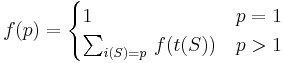
Having made this observation—and categorized all the paths—we can now count the total number of paths. Since the categories are disjoint and exhaustive, we simply add the number of paths in each category to obtain the total number of paths. But each category can be represented as a subproblem. The number of ways to go from to with the last step being from to is the same as the number of ways to go from to , period.
So we can finally conclude that the total number of ways to go from to is the sum of the number of ways to go from to for all such that we can make the trip from to in a single step (that is,  ).
).
Example
Consider the standard set of locations in the problem statement: 0, 990, 1010, 1970, 2030, 2940, 3060, 3930, 4060, 4970, 5030, 5990, 6010, 7000. Let  and
and  . The problem statement tells us that there are four ways to make the trip; we will see how to compute this number.
As indicated above, in order to count trips from 0 to 7000, we should consider all possible final legs of the trip, that is, consider every possible motel that is between 970 and 1040 km away from our final destination and assume that we will first travel there in some number of days, stay the night there, and then drive to the final destination on the final day. There are two possible motels that could come just before our final destination: the one at 5990 and the one at 6010.
By trial and error, we can determine by hand that there is one possible path that ends up at 5990, that is: 0-990-1970-2940-3930-4970-5990. There are also three possible paths that end up at 6010: 0-990-1970-2940-3930-4970-6010, 0-990-2030-3060-4060-5030-6010, 0-1010-2030-3060-4060-5030-6010. From the one path ending at 5990, we can construct one path ending at 7000 with final leg 5990, simply by appending it onto the end: 0-990-1970-2940-3930-4970-5990-7000. From the three paths ending at 6010, we can construct three paths ending at 7000 with final leg 6010, simply by appending the leg 6010-7000 to the end of each one: 0-990-1970-2940-3930-4970-6010-7000, 0-990-2030-3060-4060-5030-6010-7000, 0-1010-2030-3060-4060-5030-6010-7000. We see that all four of the paths we obtained in this way are distinct, and, furthermore, they cover all possible paths from 0 to 7000, because if we take any path from 0 to 7000, either it ends in 5990-7010 or it ends in 6010-7010, and then after removing the final leg we must get a valid path to 5990 or a valid path to 6010, and we have enumerated all of those already. We conclude that, to find the number of paths from 0 to 7000, we add the number of paths from 0 to 5990 and the number of paths from 0 to 6010. If and were different, we might have to consider a different set of penultimate destinations, but the idea is the same.
Pseudocode implementation
input n, sorted sequence x[], A, B
dp[0] ← 1                    // one way to get from x_0 to x_0, namely, by not taking any steps at all
for i ∈ [1..n]
    dp[i] ← 0
    j = i-1
    while x[i] - x[j] < A    // x_j is too close
        j = j - 1
    while x[i] - x[j] ≤ B
        dp[i] = dp[i] + dp[j]
        j = j - 1
print dp[n]
Paths in a DAG
All counting problems solvable by DP are ultimately isomorphic to the problem of counting paths in a directed acyclic graph, or DAG. This problem itself has a simple DP solution, but more complicated problems can be solved by thinking of them in this way.
Example problem: Water Park
We will start by considering the problem Water Park, which is similar to Keep On Truckin' but slightly more general. The input is a network of water slides. Each water slide connects two points, and you always slide from the higher point to the lowest point, for obvious reasons, but there may be multiple water slides that go into or come out of a single point. The problem is to determine how many different ways there are to go from the highest point (labelled 1) to the lowest point (labelled ) by sliding down the given water slides. Two ways are different if at one of them uses a slide that the other one does not use.
We solve this problem using reasoning very similar to that used in Keep on Truckin'. In order to count the number of paths from point 1 to some point  , we divide the paths into categories based on the last slide taken along the path. That is, for any given path from point 1 to point
  , we either travelled directly from point 1 to point , or we travelled from point 1 to point 2 then took a final, additional slide from point 2 to point , or we travelled from point 1 to point 3 then took a final, additional slide from point 3 to point , and so on. These categories of paths are disjoint because two paths from different categories have different final slides and therefore cannot be the same; they are exhaustive because every path from point 1 to point has to have some final slide and will hence end up in that slide's category. Finally, the size of each category is the number of paths from point 1 to the initial point of the final slide corresponding to that category.
We conclude that, in order to compute the number of paths from point 1 to point , we make a list of slides that lead directly into point , and then add up the number of paths into the initial point of each slide. Denote the initial point of a slide by  and the terminal point by
  . Thus:
We could also express this as follows:
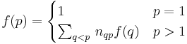
where we sum over all vertices higher (lower-numbered) than and  is the number of slides from
  to . (Note that the problem statement does not rule out multiple slides between the same pair of points!)
Example
Again, an example will help to illuminate the discussion. Suppose there are slides from 1 to 2, 1 to 3, 1 to 4, 2 to 3, 2 to 4, and 3 to 4. We want to compute the number of paths from point 1 to point 4. To do this, we first make a list of all the slides leading directly into point 4. There are three of these: 1-4, 2-4, and 3-4. Then we add the number of paths from 1 to 4 that end with the 1-4 slide, the number of paths from 1 to 4 that end with the 2-4 slide, and the number of paths from 1 to 4 that end with the 3-4 slide.
There is one path from 1 to 2: 1-2 (a single slide). We can obtain a path from 1 to 4 by adjoining 1-4, hence: 1-2-4. There are two paths from 1 to 3: 1-2-3 and 1-3; from these we obtain two paths from 1 to 4: 1-2-3-4 and 1-3-4. Finally, we shouldn't forget the direct path 1-4. We see that 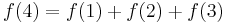 ;
;  counts the one path from 1 directly to 4,
  counts the one path from 1 to 2 then directly to 4, and
  counts the two paths from 1 to 3 and then directly to 4. This covers all possible paths from 1 to 4 with no double-counting.
Generalization
This problem may be abstracted as follows: you are given a directed acyclic graph. The network of water slides is a graph, where each point is a vertex and each slide is an edge; it is directed because you can only go one way along each edge; and it is acyclic because you cannot proceed down a sequence of slides and get back to where you started from (you will always end up somewhere lower). You want to determine how many different paths there are in this graph between a given pair of nodes, say, node  and node
  .
.
The general solution is to visit nodes in topological order from to ; that is, visit nodes in an order such that, by time time we visit a node, we have already visited all the nodes with edges leading into that node. In Water Park, this was easy: we just visit nodes in increasing numerical order. In general, this problem has disjoint and exhaustive substructure and we use the formula
where the bottom line tells to sum over all edges  into
into  ; in the summand,
  denotes the vertex that edge points away from.
Many optimization problems can be cast into a similar paradigm; here the analogous problem is finding the shortest (or longest) path between two vertices in a DAG, where each edge has some real number, its length. (Usually the problem would in fact be to find the optimal length, rather than the path itself.) We can now revisit Plentiful Paths in this light. The entire field may be considered a DAG, where each square is a vertex and there is an edge from one square to another if they are adjacent and the latter is either above or to the right of the former. Label an edge with 1 if its destination vertex contains an apple, or 0 if it does not. In this way, every possible way we can travel from the lower-left corner to the upper-right corner is assigned a weight that equals the number of apples we can collect along this path. (Actually, it will be off by one if the initial square contains an apple, but this effects only a trivial modification to the algorithm.) The problem is therefore to find the longest path between the vertices corresponding to the lower-left and upper-right squares in the DAG, and we use the formula
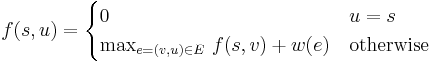
where  is the length or weight of the edge
  . To find a shortest path instead of a longest path, replace
  with
with  , or multiply all edge weights by -1. The meaning of this formula in this specific case is as follows:
  is the maximum number of apples that could've been collected by travelling from to , and is either directly below or directly to the left of , since it must be possible to travel directly from to . is 1 if there is an apple in square , and 0 otherwise. By taking the maximum value of
 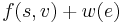 for the two possible choices of , we're selecting the predecessor square with the better optimum path (since in this case is independent of ). All this is exactly the same as in the original solution.
State and dimension
Problems that involve travelling from one place or another often obviously fall into the DAG paradigm, but the paradigm is far more general than that. Indeed, traversing a DAG topologically is the essence of DP. In all the examples we've seen so far, we would likely use an array to store the values we have computed so far. Some entries in this array depend on others, and there is usually an obvious base case (an entry we can write down trivially without examining any others) and our objective is to compute some particular entry. Of course, two entries should not depend on each other, because then we would have no way to compute either of them. This system of dependencies can be expressed by identifying each entry of the array with a vertex of the DAG and each dependency as an edge; the base case corresponds to a source of the DAG, and the final entry we want is usually a sink (since there is no point in computing additional entries that depend on the answer after we have already computed the answer).
The key to solving any problem by DP, then, is to find a useful way to construct a DAG such that each vertex's value is some function of only the values of the vertices with edges leading into it (and not the details of the path taken from the source to those vertices), and where it is simple to compute the value of the source, and, finally, where the value of the sink will be the answer to the problem instance. If the DAG is not big enough, then the rule that each vertex's value must depend only on the values of the vertices immediately before it won't be satisfied; if it's too big, then the algorithm will likely be inefficient since we need to compute the values of all (or almost all) other vertices before we can get to the value we want at the sink.
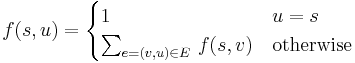
We say that we want to pick the appropriate states and transitions. A state is a vertex of the DAG, and we will usually represent it with one or more integers, indices into the array we use to do the DP. Transitions are identified with the edges leading into any given vertex, and represented by a transition function  , so that
 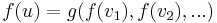 where
where  is the function we are trying to compute and
  are the vertices with an edge pointing out of them into the vertex of interest. (The case of multiple edges between a given pair of vertices is similar.) Usually, the number of states in the DP will be approximately
  for some positive integer
  , where
  is the size of the problem instance. If this is the case, we call the DP -dimensional; we will probably use a -dimensional array to store the values computed so far.