Asymptotic analysis
In theoretical computer science, asymptotic analysis is the most frequently used technique to quantify the performance of an algorithm. Its name refers to the fact that this form of analysis neglects the exact amount of time or memory that the algorithm uses on specific cases, but is concerned only with the algorithm's asymptotic behaviour—that is, how the algorithm performs in the limit of infinite problem size.
Contents
Irrelevance of constant factor
It does this by neglecting the so-called invisible constant factor. The reasoning is as follows. Suppose Alice and Bob each write a program to solve the same task. Whenever Alice's program and Bob's program are executed with the same input on a given machine (which we'll call ALOPEX), Alice's program is always about 25% faster than Bob's program. The table below shows the number of lines of input in the first column, the execution time of Alice's program in the second, and the execution time of Bob's program in the third:
| N | Alice | Bob |
|---|---|---|
| 104 | 0.026 | 0.032 |
| 105 | 0.36 | 0.45 |
| 106 | 3.8 | 4.7 |
Practically speaking, Alice's program is faster. In theory, however, the two programs have equally efficient algorithms. This is because an algorithm is an abstraction independent of the machine on which it runs, and we could make Bob's program just as fast as Alice's by running it on a computer that is 25% faster than the original one.
If this argument sounds unconvincing, consider the following argument. Programs, as they run on real machines, are built up from a series of very simple instructions, each of which is executed in a period of time on the order of a nanosecond on a typical microcomputer. However, some instructions happen to be faster than others.
Now, suppose we have the following information:
- On ALOPEX, the
MULTIPLYinstruction takes 1 nanosecond to run whereas theDIVIDEinstruction takes 2 nanoseconds to run. - We have another machine, which we'll call KITSUNE, on which these two instructions both take 1.5 nanoseconds to run.
- When Bob's program is given 150000 lines of input, it uses 1.0×10⁸ multiplications and 3.0×10⁸ divisions, whereas Alice's program uses 4.0×10⁸ multiplications and 0.8×10⁸ divisions on the same input.
Then we see that:
- On ALOPEX, Bob's program will require (1 ns)×(1.0×10⁸) + (2 ns)×(3.0×10⁸) = 0.70 s to complete all these instructions, whereas Alice's program will require (1 ns)×(4.0×10⁸) + (2 ns)×(0.8×10⁸) = 0.56 s; Alice's program is faster by 25%.
- On KITSUNE, Bob's program will require (1.5 ns)×(1.0×10⁸) + (1.5 ns)×(3.0×10⁸) = 0.60 s, whereas Alice's will require (1.5 ns)×(4.0×10⁸) + (1.5 ns)×(0.8×10⁸) = 0.72 s. Now Bob's program is 20% faster than Alice's.
Thus, we see that a program that is faster on one machine is not necessarily faster on another machine, so that comparing exact running times in order to decide which algorithm is faster is not meaningful.
The same can be said about memory usage. On a 32-bit machine, an int (integer data type in the C programming language) and an int* (a pointer to an int) each occupy 4 bytes of memory, whereas on a 64-bit machine, an int uses 4 bytes and an int* uses 8 bytes; so that an algorithm that uses more pointers than integers may use more memory on a 64-bit machine and less on a 32-bit machine when compared to a competing algorithm that uses more integers than pointers.
Why the machine is now irrelevant
The preceding section should convince you that if two programs's running times differ by at most a constant factor, then their algorithms should be considered equally efficient, as we can make one or the other faster in practice just by designing our machine accordingly. Let's now consider a case in which one algorithm can actually be faster than another.
Suppose that Alice and Bob are now given a new problem to solve and their algorithms perform as follows on ALOPEX:
| N | Alice | Bob |
|---|---|---|
| 103 | 0.040 | 0.0013 |
| 104 | 0.38 | 0.13 |
| 105 | 3.7 | 12 |
| 106 | 37 | 1500 |
Observe that when we multiply the problem size by 10, Alice's program takes about 10 times longer, but Bob's program takes about 100 times longer. Thus, even though Bob's program is faster than Alice's program for small inputs (10000 lines or fewer), in the limit of infinite problem size, Alice's program will always be faster. Even if we run Bob's program on a supercomputer and Alice's program on a 386, for sufficiently large input, Alice's program will always finish first, since no matter how much of a disadvantage Alice's program has, it catches up more and more as we increase the problem size; it scales better than Bob's algorithm.
Also observe that Alice's algorithm has running time approximately proportional to the size of its input, whereas Bob's algorithm has running time approximately proportional to the square of the size of its input. We write that Alice's algorithm has running time  whereas Bob's has running time
  . Notice that we don't bother to write the constant factor, since this varies from machine to machine; we write only the part that tells us how the algorithm scales. Since
  grows much more quickly than
  as increases, we see that Bob's algorithm is slower than Alice's.
Asymptotic optimality
An algorithm is said to be asymptotically optimal when it is the best-performing algorithm possible for a given problem, usually in terms of running time. There may be multiple asymptotically optimal algorithms for a given problem; for example, Tarjan's algorithm, Gabow's algorithm, and Kosaraju's algorithm are all asymptotically optimal for finding strongly connected components in a graph.
A program that uses an asymptotically optimal algorithm may not be the fastest (or least memory-hungry, etc.) program possible. For example, a program that uses Kosaraju's algorithm might be outperformed by a program that uses Tarjan's algorithm. However, it is possible to beat the performance of a program that uses an asymptotically optimal algorithm by at most a constant factor. Furthermore, if an algorithm is not asymptotically optimal, then, given large enough input size, it will always be outperformed by an asymptotically optimal algorithm.
Asymptotic complexity
The performance of an algorithm in the limit of infinite problem size is called its asymptotic complexity, or just complexity. This may be subdivided into space complexity, time complexity, and so on. The complexity of a problem is defined to be the complexity of the optimal algorithm that solves it. Problems may be divided into complexity classes based on their complexities.
Determining a problem's asymptotic complexity is important in theoretical computer science; there are many problems (such as matrix multiplication) whose complexities remain unknown. Often, a computer scientist will discover an algorithm for a problem and then show that it is asymptotically optimal; this is usually considered a landmark result in the study of that problem. More rarely, one will prove that an algorithm exists for a given problem, and show that it is asymptotically optimal, without actually giving the algorithm (nonconstructive proof).
Notation
We are now ready to give an explanation of the  -notation used in the previous section. (See section Big theta notation below.) We suppose that functions
  and
and  map the positive integers to the positive real numbers. The interpretation is that
  represents the amount of time (in some units) that it takes a certain algorithm to process an input of size
  when run on a certain machine.
Big O notation
We say that  when
when  is asymptotically at least as large as . This is read f is big-O of g. Mathematically, this is defined to mean that there are some constants
  such that
  for all
  ; to read it idiomatically, for sufficiently large , is bounded by a constant times .
This means that if we plotted and on the same set of axes, with along the positive x-axis, then we can scale the curve such that it always lies above the curve .
For example, if we plot  and
and  on the same set of axes, then we see that by scaling by a factor of
  , we can make the curve of lie above the curve of . Therefore,
  .
.
Similarly, if we plot  and
and  on the same set of axes, and we scale by a factor of 5, we will make the curve of lie above the curve of . So
  .
.
On the other hand, if  and
and  , no matter how much we scale , we cannot make it lie above . We could for example try scaling by a factor of 100. Then, we will have
  for all up to 500, but for
  , will be larger. If we try scaling by a factor of 1000, then will still catch up at
  , and so on. So
  .
.
Big O notation is the most frequently used notation for describing an algorithm's running time, since it provides an upper bound. If, for example, we write that an algorithm's running time is  , then this is a guarantee that, as grows larger, the relative increase in the algorithm's running time is at most that of
  , so that when we double , our algorithm's running time will be at most quadrupled, and so on. This characterization is machine-independent; if an algorithm is on one machine then it will be on any other machine as well. (This holds true under the assumption that they are both classical von Neumann machines, which is the case for all computing machines on Earth right now.)
An algorithm that is  for some constant
  is said to be polynomial-time; its running time is bounded above by a polynomial in its input size. Polynomial-time algorithms are considered "efficient", because they provide the guarantee that as we double the problem size, the running time increases by a factor of at most
  . If an algorithm is not polynomial-time, it could be that doubling the problem size from 1000 to 2000 increases the running time by a factor of 10, but doubling the problem size from 10000 to 20000 increases the running time by a factor of 100, and the factor becomes worse and worse as the problem size increases; these algorithms are considered inefficient. The first polynomial-time algorithm discovered that solves a particular problem is usually considered a breakthrough.
Big omega notation
Big omega notation is the opposite of big O notation. The statement that is equivalent to the statement that  . Conceptually, it means that is asymptotically at least as large as . Therefore, big omega notation provides a lower bound, instead of an upper bound. For example, if an algorithm's running time is
  for some
  , then when we increase the problem size from to
  , the running time of our algorithm will increase by a factor of at least
  . Approximately doubling the input size will then approximately square the running time. This scaling behaviour, called exponential time, is considered extremely inefficient.
Big theta notation
If and  , then and differ by only a constant factor from each other, like the running time of Alice and Bob's algorithms from the first section. In this case, we write
  or equivalently
  . Whereas big O notation gives us an upper bound on a function, such as an algorithm's running time as a function of its input size, and big omega notation gives us a lower bound, big theta notation gives us both simultaneously—it gives us an expectation of that function. This is often expressed as f is on the order of g.
Thus, if an algorithm's running time is  , and we double the input size , then we have an expectation that the running time of the algorithm will be nearly exactly four times what it was before, whereas big O notation would only tell us that it is not more than four times greater, and big omega notation that it is at least four times greater.
Little O notation
Whereas the big O notation expresses that grows at least as quickly as in an asymptotic, constant-factor-oblivious sense, little O notation, as in  , expresses that grows strictly more quickly than in the limit of infinite . It means that
  . This notation is not used very often in computer science (simply because it is rarely useful). Additionally, the limit based notation is not entirely equivalent to the big/little-Oh notation since the limit of the quotient might not exist in case of non-continuous functions such as the step function, etc...
Little omega notation
Little omega notation is the opposite of little O notation; the statement that is equivalent to the statement that  . Little omega notation, like little O notation, is rarely used in computer science.
Proper use of notation
In the five notations above, note the use of the  symbol. The expression is sometimes written as
  . This is incorrect. The symbol
  is not a function, but a set of functions; it is the set of all functions whose growth is bounded by a constant factor of in the infinite limit, as defined above. Use of the equal sign would suggest that we could flip it around to get
  , but this would not make any sense.
It is fine to read as f of n is O g of n, but important to remember that the word "is" does not denote equality.
Tilde/swung dash
The notation  means that
  . This is usually not used when discussing running times of algorithms, because it does not ignore the constant factor the way that the other notations do; hence
  but
but  . On the other hand,
  . However, this notation may be useful when we care about the constant factor because we are quantifying something that depends on only the algorithm itself instead of the machine it runs on. For example, the amount of time an algorithm uses to sort its input depends on what machine it runs on, but the number of comparisons that the algorithm uses for a given input does not depend on the machine. In this case we might say that one algorithm requires
  comparisons, whereas another requires
  comparisons. Both algorithms are
  , but the tilde notation distinguishes their performance.
Mathematical discussion
The following identities hold. The proofs are left as an exercise to the reader.
Relationships between notations
- if and only if
- if and only if
- if and only if and
- implies
-
 implies
 - implies
- implies
- implies
- is equivalent to
Reflexivity, symmetry, and transitivity
Reflexivity
-
 .
. -
 .
. -
 .
. -
 .
. -
 .
. -
 .
.
Symmetry
- is equivalent to .
- is equivalent to
 .
. - implies
 .
. - implies
 .
.
Transitivity
- If and
 then
then  .
. - If and
 then
then  .
. - If and
 , then
  .
. - If and
 then
then  .
. - If and
 then
then  .
. - If and
 then
then  .
.
Mixed transitivity
- If and , then .
- If and , then .
- If and , then .
- If and , then .
- If and , then .
- If and , then .
Composition
- TODO
Hierarchy of functions in one variable
From the reflexivity, symmetry, and transitivity properties above, it can be seen that defines an equivalence relation on functions from  to
to  . Thus and
  belong to the same equivalence class, but neither belongs to the same equivalence class as
  . The equivalence class a function belongs to in this context is called its order. Notably,
  for any
  , so scaling a function does not change its order.
These orders may in turn be ranked. If , then , in a sense, increases strictly more quickly than , and furthermore every function of 's order increases strictly more quickly than every function of 's order, because of the mixed transitivity relations given above.
(Note that in the below, the term "order" will be used in two different senses.)
The orders may then be partially ordered, where we define ![[f] \leq [g]](/wiki/images/math/c/3/8/c3856bf4b5d84fea4141c9031d0e10cb.png) if and only if . They cannot be totally ordered, because it is possible to define functions and such that
if and only if . They cannot be totally ordered, because it is possible to define functions and such that  and
and  , so that
 ![[f] \nleq [g]](/wiki/images/math/e/f/f/eff7028e4d1e71c1af5c08a24b2e5880.png) and
and ![g \nleq [f]](/wiki/images/math/7/4/3/743be617f60e03812dd7d3c0a7f09383.png) . How to do this is left as an exercise to the reader. The vast majority of orders encountered in the analysis of algorithms, however, belong to a chain (are totally ordered). Here is a list of orders of functions, with the more quickly growing functions toward the end. Names are given for common orders of complexity, so that, for example, an algorithm requiring about
. How to do this is left as an exercise to the reader. The vast majority of orders encountered in the analysis of algorithms, however, belong to a chain (are totally ordered). Here is a list of orders of functions, with the more quickly growing functions toward the end. Names are given for common orders of complexity, so that, for example, an algorithm requiring about  steps (with
  constant) to process an input of size is said to require linear time. The term linear space is defined analogously.
- Constant:
 (Example: Time required to add a node to the front of a linked list)
 - Inverse Ackermann function:
 (Example: Amortized time required to perform a disjoint set operation)
 - Iterated logarithm:
- Doubly logarithmic:
 (Example: Average running time of interpolation search)
 - Logarithmic:
 (Example: Time required by binary search)
- Note that
 belongs to this class regardless of the value of
  . That is,
  for any
  . This is because of the relation
  , where the denominator is a constant. This is why one sees "the running time of such-and-such algorithm is
  " without any base stated, or that it is
  even though the analysis clearly suggests about
  steps.
- Note that
- Polylogarithmic:
- There is a separate order for each value of ;
 .
.
- There is a separate order for each value of
-
 for
for 
- There is a separate order for each value of ;
 .
.
- There is a separate order for each value of
- Linear:
 (Example: Time required to search for an item in an unsorted list)
 -
 (Example: Time required to sort an array of items using only comparisons and swaps)
- The name "linearithmic" has been proposed for this complexity. Notably, a former PEG leader has dismissed it as ridiculous and fake-sounding. "Log-linear" is also a possible name.
- The function
 also belongs to this class.
-
 (Example: Space required by high-dimensional geometric segment trees)
 - Quadratic: (Example: Time required to find a minimum spanning tree in a dense graph of vertices)
- Every quadratic polynomial belongs to this class, regardless of its coefficients.
- Cubic:
 (Example: Time required by the Floyd–Warshall algorithm)
- Every cubic polynomial belongs to this class, regardless of its coefficients.
- Exponential:
 , for
, for  (Example: Naive brute-force solution to subset sum problem)
- There is a separate order for each value of ;
 .
.
- There is a separate order for each value of
- Factorial:

-

- Doubly exponential:
 (usually
  )
)
Revisiting identities
Some of the identities given above, especially the mixed transitivity identities, are much simplified if we consider:
- to be equivalent to
- to be equivalent to
![[f] \geq [g]](/wiki/images/math/3/0/6/306e0c3b46e984b5d50b715ada541530.png)
- to be equivalent to
![[f] < [g]](/wiki/images/math/f/1/9/f198e9a7f948d4384e05f225b5460757.png)
- to be equivalent to
![[f] > [g]](/wiki/images/math/c/c/4/cc4a24cfa212a2d17304c81c126f435b.png)
- to be equivalent to
![[f] = [g]](/wiki/images/math/4/6/6/46691983add002759ec9845017a9a9e4.png)
For example, the arithmetic identity that  and
and  imply
imply  suggests the identity that if and , then .
Multiple variables
When the running time or space usage of an algorithm depends on more than one parameter (which is especially common in graph theory, where both the number of vertices  and the number of edges
  are important), the use of big O notation and its brethren becomes tricky. For example, if a geometric algorithm involving points in
  -dimensional space had running time
  , then one might sometimes express this as simply
  and call it linear (because the reader is supposed to understand that is being held constant). However, this does not adequately capture the essence of the algorithm's time complexity, which is linear in but exponential in .
It would, in this case, be advisable to avoid causing confusion by always writing it as or  , rather than as "" or "linear", unless it is very clear from context that is being held constant.
With two variables, the notation  means that there exist
  such that
  whenever and
  . Big omega and big theta notation on multiple variables are defined analogously. (The other three notations are trickier to define in this case, since they involve limiting processes, and multivariate limits are tricky.) Here, we should write fully instead of simply
  , so we always know what the relevant variables are.
How to analyze an algorithm
In both theory and practice, it is important to be able to determine the complexity of an algorithm.
In theory, much of computer science is the quest for better and better complexities of algorithms for solving various problems. This is often true even when the algorithm that is better in theory is worse in practice. For example, Strassen multiplication has a complexity of  , which is better than the naive method's
  , but only outperforms the naive method in practice for very large matrices.
In practice, an upper bound on an algorithm's time or memory usage in terms of big O notation is an indication of how well it scales. An algorithm that takes time to search for an article in a database of articles, for example, would probably work fine for this wiki, but would be horrendously inefficient for Wikipedia's purposes; scales much better in the sense that doubling the number of articles would only add a constant to the amount of time required per search.
Complexities in contests
Around the turn of the century, the International Olympiad in Informatics underwent a massive increase in difficulty as well as a fundamental shift in problem style. In the nineties, IOI problems often required recursive backtracking searches that had to be cleverly optimized by pruning in order to find an optimal solution within the time limit. After the shift, however, most problems required knowledge of algorithms typically taught in college computer science courses, which, when carefully composed, would give an asymptotically optimal algorithm for the overall problem.
With the older problems, it is not easy to predict theoretically what the running time should be, so one must take recourse to simply coding a solution, testing it on large test cases, and then optimizing it further if it does not pass the largest possible test cases in time. With the newer problems, on the other hand, one can often guess at what an acceptable time complexity would be simply by examining the bounds given.
As a rule of thumb for olympiad-style contests:
- An exponential-time algorithm (
 ) suffices to tackle test cases with
  , so a bound this small suggests an exponential-time algorithm. Dynamic programming is often required to achieve this time bound, or a polynomial multiple of it, rather than
  , which is too slow.
 - A cubic-time algorithm will suffice for up to about 300.
- A quadratic-time algorithm will suffice for up to about 5000.
- An
 time algorithm will suffice for up to about 200000. The number 100000 is a very common bound on input size in olympiad problems, and almost always suggests that a contestant should aim to invent an algorithm with time complexity of around . (This aspect of olympiad contests has been criticized.)[1] is almost always too slow in this case.
 - A linear-time algorithm is typically required if the input can be even larger than this, usually 300000 or more lines.
Best case, average case, and worst case
The running time of an algorithm usually depends on not only the size of input (number of characters in a string, length of a number's binary representation, number of edges in a graph, etc.) but also the details. For example, bubble sort requires only linear time to sort an array that is already sorted, but quadratic time to sort an array that is sorted in reverse order initially. These are called the best case and worst case, respectively, for bubble sort, since they represent the best and worst that bubble sort can perform on an input of a given size.
Theoreticians usually focus on optimizing the worst-case running time of an algorithm. In practice, the worst case is important, but the average case is also important. The average case running time is defined as the expected running time for the algorithm assuming that its input is of a given size and drawn randomly and uniformly from the set of all possible inputs of that size. The average case tends to be more difficult to mathematically analyze than the worst case. As an example, quicksort is in both the average case and the best case, but in the worst case, so it is often used in practice (such as in the std::sort implementation in libstdc++) with a fallback to heapsort to handle particularly bad cases. (This combination is called introsort.)
In contests, the worst case is more important than the average case, because it is almost guaranteed that the problem setters will include contrived input—input that is intended to be the worst case for a typical "easy" algorithm, in order to separate contestants who implement this algorithm from cleverer contestants who implement an algorithm with better worst-case performance.
In time-critical applications (with an obvious and very cliché example being the software that controls space shuttles), the worst case is the only case that matters; catastrophic failure could occur if an algorithm with poor worst-case performance were to hit the worst case "on the job".
The best-case complexity is usually not considered very important, whether in theory or in practice.
The worst-case and average-case complexity of an algorithm are often similar, or even of exactly the same order. The best-case complexity is usually significantly better. Bubble sort is given above as an example; its average case complexity is quadratic, the same as its worst-case complexity. Another example is searching for a key in a balanced binary search tree, which is logarithmic time in the average and worst case but constant time in the best case.
Time versus space
It is usually very easy to analyze the space complexity of an algorithm, in contrast to its time complexity, which is usually trickier. An interesting example is that of the disjoint sets data structure. It obviously requires linear space (simply an array for each item that stores the ID of its parent item in its tree), but the analysis of its time complexity is beyond the scope of a typical undergraduate computer science course.
We will focus on computing time complexity for the remainder of this article. If an algorithm or data structure's space complexity is difficult to analyze, it may be specially treated on its own page.
Instruction counting: the basic idea
The most basic way to analyze the time complexity of an algorithm is by supposing that certain instructions take constant time to execute and then counting the number of such instructions that the algorithm uses. Most commonly:
- A scalar variable (a variable that requires a constant amount of memory to store), which is generally a character, an integer, a floating point number, a Boolean variable, or a pointer, takes constant time to read from input, write to output, or copy from one memory location to another.
- Dynamically allocating or disposing of enough memory to store one scalar variable takes constant time.
- Comparing two scalar variables (to determine whether the first is less than, equal to, or greater than the second) takes constant time.
- A Boolean function (AND, OR, XOR, NOT) requires constant time to compute.
- Every arithmetic operation takes constant time, as does every bitwise operation (such as a left shift).
- Every standard mathematical operation then also takes constant time, since we only need to compute its value to limited precision, and can thus approximate it using a certain number of arithmetic operations.
- Jumping from one place in the code to another takes constant time; this includes exiting a loop or subroutine, or choosing a branch of an if statement after the condition has already been checked.
- Dereferencing a pointer takes constant time.
- Accessing the ith element of an array, given i, takes constant time (random access machine model).
We don't have to count exactly how many instructions the CPU will execute in performing our algorithm; we just have to get it right to within a constant factor.
Simple examples
It then follows that:
- A block of code that involves at most a constant number of constant-time instructions takes constant time to execute.
If the number of instructions required by an algorithm is some polynomial in its input size , then only the leading term is significant (and its coefficient doesn't matter). For example, if an algorithm requires  constant-time instructions, then it requires time. This is a simple consequence of the fact that
  , so that
  , thus
  . This is true even of functions that are linear combinations of powers of but are not polynomials (because the exponents are negative or fractional).
- A loop whose body contains only a constant number of constant-time instructions, and whose termination condition takes constant time to check, and runs times, requires time. This is because the body requires linear time in total across all iterations, checking the condition also requires linear time, and exiting the loop via a jump requires constant time; and the constant term is not significant compared to the linear term.
- Copying an array of elements or copying a string of characters takes time.
- Lexicographically comparing two strings takes constant time in the best or average case, and linear time in the worst case.
- Adding or subtracting two large integers, each of size , takes time, using the traditional carrying and borrowing-based algorithms.
- When we say that an integer is of size , we mean that it is so large that it can't fit in a single scalar variable, but instead requires scalar variables to contain it. In Java, for example, an
intis a scalar variable, whereas aBigIntegeris not. See big numbers for more information.
- When we say that an integer is of size
- Copying an array of
- A loop whose body contains only a constant number of constant-time instructions, and runs
 times, requires time to complete. This is because constant terms are insignificant compared to logarithmic terms, as
  . It follows that binary search on an array of scalar variables takes logarithmic time.
 - If we have two nested loops, one which times and one of which runs times, and the conditions and body each only take constant time to evaluate once, then this nested loop structure takes
 time. This result easily extends to a nested structure of more than two loops.
- Multiplying together two large integers of size using the "longhand" method taught in elementary school requires time.
- The Floyd–Warshall algorithm, which consists of three nested loops, each of which runs times, and whose inner body contains only a constant number of constant-time instructions, takes
 time.
time.
- Multiplying together two large integers of size
Recursive functions
Many algorithms work by breaking the input down into smaller pieces, recursively solving each smaller piece as though it were an independent problem, and then combining the results to obtain a solution to the original instance. This algorithmic paradigm is known as divide and conquer, and its running time is usually analyzed slightly differently from that of the simpler algorithms from the previous section.
Examples:
- Merge sort, which sorts a list by dividing it into two sub-lists, sorting each sub-list, and then merging the two sorted sub-lists to obtain the original list, sorted. The merge step takes time if the original list had elements. The overall running time is .
- Karatsuba multiplication, which multiplies two -digit numbers (see Big numbers) by dividing each number into two halves and recursively multiplying three pairs of halves, along with some additions and subtractions which take time in total. The overall running time is
 .
. - One solution to the closest pair of points problem finds the closest pair by dividing the point set with a half plane to obtain two sets of points of approximately half the size, finding the closest pair of points within each set, and then sorting points close to the dividing line and sweeping to find the closest pair across the division, which takes time (for the sorting). The overall running time is then
 . (NB: This can be improved to if we concomitantly run merge sort, rather than re-sorting along the dividing line in each step.)
How do we analyze the running time of such algorithms? We can reason as follows:
- In the case of merge sort, we start out with one instance (the original list of size ), which gives rise to two subinstances of size
 ; these in turn give rise to a total of four subinstances of size
  , and so on down to subinstances of size 1 or 2. There are about
  "levels" to this scheme, and at each level, we have about subinstances of size
  , and a linear amount of work is required in the "conquer" step of each; so that is about steps at each level, or about
  steps in total, giving .
 - In Karatsuba multiplication, there will again be about levels. On the topmost level, we have one instance with size . On the next level, we have three instances with size , and then nine instances with size , and so on down. A linear amount of additional work is required for the "conquer" step for each instance, so that is about work on the topmost level, about
 on the next level, and so on down. So the total running time will be about
 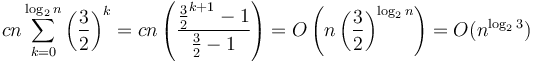 . (Several steps were omitted.)
 - In the third algorithm listed above, there are again about levels; on the topmost level, the work done is ; then
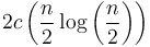 on the next level, since we will have two subinstances of size
  , which will each require
 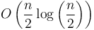 work; then on the next level,
 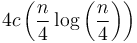 , and so on down; the total work done is about
 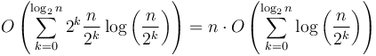 . This gives us an arithmetic series, with first term (here
  ) and last term about 0 (for when
 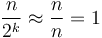 since
since  ) and a total of about terms; its sum is then about
  giving overall.
We would like to have some way to tackle the general case, without so much messy mathematical reasoning in each individual case. By general case, we mean that we assume that to solve an instance of size using some algorithm, we divide it into chunks of size about  , and solve
  subproblems using those chunks, along with extra work in the amount of , unless
  for some constant , which represents a base case that can be solved in
  time. For example, in the first of the three examples above, we have
 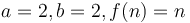 ; in the second,
 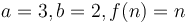 , and in the third,
  .
.
The master theorem
The authoritative statement of the master theorem is from CLRS[2]. Suppose that  and
and  above, and is positive. Then, there are three cases:
- If
 for some
  , then the overall running time is
  .
. - If
 , for some
  , then the overall running time is
  .
. - If
 for some , and, furthermore,
 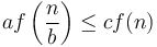 for some
  and all sufficiently large , then the overall running time is
  .
.
For example, Karatsuba multiplication falls into the first case, since and 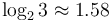 . The theorem then tells us that the overall running time is . What is happening here is that as we proceed from one level to the next, the amount of work done on the current level increases exponentially or faster. In this particular case, each level entails 1.5 times as much work as the previous level. Intuitively, this means most of the work is done on the lowest level, on which we have subproblems, each with size 1. The earlier analysis then applies. The reason why we need is precisely to ensure this exponential growth. If is exactly
  , then we will have
  , that is, the amount of work done on each level will be the same. But if grows more slowly than this, then will be less than
  . If it grows polynomially more slowly (that is, by a factor of
  or more), then the desired exponential growth will be attained.
Merge sort and the closest pair of points algorithm are covered by case 2. For merge sort, we have (there is no log factor at all). Here the time spent on each level is the same, since  if
if  , so we simply multiply by the number of levels, that is,
  . For the closest pair of points algorithm, we have
  . When
  , then there is a decrease in the amount of work done as we go further down, but it is slower than an exponential decay. In each case the average amount of work done per level is on the order of the amount of work done on the topmost level, so in each case we obtain
  time.
time.
Case 3 is not often encountered in practice. When  (with
(with  ), there is an exponential (or faster) decay as we proceed from the top to the lower levels, so most of the work is done at the top, and hence the behaviour is obtained. The condition that is not actually needed in the statement of Case 3, since it is implied by the condition that . The reason why the theorem is stated as it is above is that if is actually of the form
  , which covers most of the cases, then the other condition is implied, and we don't need to explicitly check it, but can instead just look at the form of . However, there are some possibilities for that are not "well-behaved", and will not satisfy the condition .
An actual proof of the master theorem is given in CLRS.
Akra–Bazzi theorem
TODO
Amortized analysis
TODO
References
- ↑ Ribiero, P. and Guerreiro, P. Improving the Automatic Evaluation of Problem Solutions in Programming Contests. Olympiads in Informatics, 2009, Vol. 3, 132–143. Retrieved from http://www.mii.lt/olympiads_in_informatics/pdf/INFOL048.pdf
- ↑ Thomas H. Cormen, Charles E. Leiserson, Ronald L. Rivest, and Clifford Stein. Introduction to Algorithms, Second Edition. MIT Press and McGraw-Hill, 2001. ISBN 0-262-03293-7. Sections 4.3 (The master method) and 4.4 (Proof of the master theorem), pp. 73–90.