Convex hull trick
The convex hull trick is a technique (perhaps best classified as a data structure) used to determine efficiently, after preprocessing, which member of a set of linear functions in one variable attains an extremal value for a given value of the independent variable. It has little to do with convex hull algorithms.
Contents
History
The convex hull trick is perhaps best known in algorithm competitions from being required to obtain full marks in several USACO problems, such as MAR08 "acquire", which began to be featured in national olympiads after its debut in the IOI '02 task Batch Scheduling, which itself credits the technique to a 1995 paper (see references). Very few online sources mention it, and almost none describe it. It has been suggested (van den Hooff, 2010) that this is because the technique is "obvious" to anybody who has learned the sweep line algorithm for the line segment intersection problem.
The problem
Suppose that a large set of linear functions in the form  is given along with a large number of queries. Each query consists of a value of
  and asks for the minimum value of
  that can be obtained if we select one of the linear functions and evaluate it at . For example, suppose our functions are
  ,
,  ,
,  , and
, and  and we receive the query
  . We have to identify which of these functions assumes the lowest -value for , or what that value is. (It is the function , assuming a value of 2.)
The variation in which we seek the maximal line, not the minimal one, is a trivial modification and we will focus our attention on finding the minimal line.
When the lines are graphed, this is easy to see: we want to determine, at the -coordinate 1 (shown by the red vertical line), which line is "lowest" ( has the lowest -coordinate). Here it is the heavy dashed line, .
Naive algorithm
For each of the  queries, of course, we may simply evaluate every one of the linear functions, and determine which one has the least value for the given -value. If
  lines are given along with queries, the complexity of this solution is
  . The "trick" enables us to speed up the time for this computation to
  , a significant improvement.
The technique
Consider the diagram above. Notice that the line will never be the lowest one, regardless of the -value. Of the remaining three lines, each one is the minimum in a single contiguous interval (possibly having plus or minus infinity as one bound). That is, the heavy dotted line is the best line at all -values left of its intersection with the heavy solid line; the heavy solid line is the best line between that intersection and its intersection with the light solid line; and the light solid line is the best line at all -values greater than that. Notice also that, as increases, the slope of the minimal line decreases: 2/3, -1/2, -3. Indeed, it is not difficult to see that this is always true.
Thus, if we remove "irrelevant" lines such as in this example (the lines which will never give the minimum -coordinate, regardless of the query value) and sort the remaining lines by slope, we obtain a collection of  intervals (where is the number of lines remaining), in each of which one of the lines is the minimal one. If we can determine the endpoints of these intervals, it becomes a simple matter to use binary search to answer each query.
Etymology
The term convex hull is sometimes misused to mean upper/lower envelope. If we consider the "optimal" segment of each of the three lines (ignoring ), what we see is the lower envelope of the lines: nothing more or less than the set of points obtained by choosing the lowest point for every possible -coordinate. (The lower envelope is highlighted in green in the diagram above.) Notice that the set bounded above by the lower envelope is convex. We could imagine the lower envelope being the upper convex hull of some set of points, and thus the name convex hull trick arises. (Notice that the problem we are trying to solve can again be reformulated as finding the intersection of a given vertical line with the lower envelope.)
Adding a line
As we have seen, if the set of relevant lines has already been determined and sorted, it becomes trivial to answer any query in  time via binary search. Thus, if we can add lines one at a time to our data structure, recalculating this information quickly with each addition, we have a workable algorithm: start with no lines at all (or one, or two, depending on implementation details) and add lines one by one until all lines have been added and our data structure is complete.
Suppose that we are able to process all of the lines before needing to answer any of the queries. Then, we can sort them in descending order by slope beforehand, and merely add them one by one. When adding a new line, some lines may have to be removed because they are no longer relevant. If we imagine the lines to lie on a stack, in which the most recently added line is at the top, as we add each new line, we consider if the line on the top of the stack is relevant anymore; if it still is, we push our new line and proceed. If it is not, we pop it off and repeat this procedure until either the top line is not worthy of being discarded or there is only one line left (the one on the bottom, which can never be removed).
How, then, can we determine if the line should be popped from the stack? Suppose  ,
,  , and
, and  are the second line from the top, the line at the top, and the line to be added, respectively. Then, becomes irrelevant if and only if the intersection point of and is to the left of the intersection of and . (This makes sense because it means that the interval in which is minimal subsumes that in which was previously.) We have assumed for the sake of simplicity that no three lines are concurrent.
Analysis
Clearly, the space required is  : we need only store the sorted list of lines, each of which is defined by two real numbers.
The time required to sort all of the lines by slope is  . When iterating through them, adding them to the envelope one by one, we notice that every line is pushed onto our "stack" exactly once and that each line can be popped at most once. For this reason, the time required overall is for this step; although each individual line, when being added, can theoretically take up to linear time if almost all of the already-added lines must now be removed, the total time is limited by the total number of times a line can be removed. The cost of sorting dominates, and the construction time is
Case study: USACO MAR08 acquire
Problem
Up to 50000 rectangles of possibly differing dimensions are given and it is desired to acquire all of them. To acquire a subset of these rectangles incurs a cost that is proportional to neither the size of the subset nor to its total area but rather the product of the width of the widest rectangle in the subset times the height of the tallest rectangle in the subset. We wish to cleverly partition the rectangles into groups so that the total cost is minimized; what is the total cost if we do so? Rectangles may not be rotated; that is, we may not interchange the length and width of a rectangle.
Observation 1: Irrelevant rectangles
Suppose that both of rectangle A's dimensions equal or exceed the corresponding dimensions of rectangle B. Then, we may remove rectangle B from the input because its presence cannot affect the answer, because we can merely compute an optimal solution without it and then insert it into whichever subset contains rectangle A without changing the cost. Rectangle B, then, is irrelevant. We first sort the rectangles in ascending order of height and then sweep through them in linear time to remove irrelevant rectangles. What remains is a list of rectangles in which height is monotonically increasing and width is monotonically decreasing. (Otherwise, a contradiction would exist to our assumption that all irrelevant rectangles have been removed.)
Observation 2: Contiguity
In the sorted list of remaining rectangles, each subset to be acquired is contiguous. Thus, for example, if there are four rectangles, numbered 1, 2, 3, 4 according to their order in the sorted list, it is possible for the optimal partition to be  but not
  ; in the latter,
  is contiguous but
  is not. This is true because, in any subset, if rectangle A is the tallest and rectangle B is the widest, then all rectangles between them in the sorted list may be added to this subset without any additional cost, and therefore we will always assume that this occurs, making each subset contiguous.
DP solution
The remaining problem then is how to divide up the list of rectangles into contiguous subsets while minimizing the total cost. This problem admits a  solution by dynamic programming, the pseudocode for which is shown below: Note that it is assumed that the list of rectangles comes "cooked"; that is, irrelevant rectangles have been removed and the remaining rectangles sorted.
input N
for i ∈ [1..N]
     input rect[i].h
     input rect[i].w
let cost[0] = 0
for i ∈ [1..N]
     let cost[i] = ∞
     for j ∈ [0..i-1]
         cost[i] = min(cost[i],cost[j]+rect[i].h*rect[j+1].w)
print cost[N]
In the above solution, cost[k] stores the minimum possible total cost for acquiring the first k rectangles. Obviously, cost[0]=0. To compute cost[i] when i is not zero, we notice that it is equal to the total cost of acquiring all previous subsets plus the total cost of acquiring the subset containing rectangle number i; the latter may be readily calculated if the size of the latter subset is known, because it is merely the width of the first times the height of the last (rectangle number i). We wish to minimize this, hence cost[i] = min(cost[i],cost[j]+rect[i].h*rect[j+1].w). (Notice that j is the last rectangle of the previous subset, looping over all possible choices.)
Unfortunately, is too slow when  , so a better solution is needed.
Observation 3: Convexity
Let ![m_j=\mathrm{rect}[j+1].w](/wiki/images/math/3/c/4/3c401198348a95bd88ccc5a1383c9642.png) ,
, ![b_j=\mathrm{cost}[j]](/wiki/images/math/f/3/3/f330aa433eeaad03088a2adf235c0b64.png) , and
, and ![x=\mathrm{rect}[i].h](/wiki/images/math/2/c/a/2ca9b1006186905dfccd16bb2662862d.png) . Then, it is clear that the inner loop in the above DP solution is actually trying to minimize the function
. Then, it is clear that the inner loop in the above DP solution is actually trying to minimize the function  by choosing
  appropriately. That is, it is trying to solve exactly the problem discussed in this article. Thus, assuming we have implemented the lower envelope data structure discussed in this article, the improved code looks as follows:
input  N
for i ∈ [1..N]
     input rect[i].h
     input rect[i].w
let E = empty lower envelope structure
let cost[0] = 0
add the line y=mx+b to E, where m=rect[1].w and b=cost[0] //b is zero
for i ∈ [1..N]
     cost[i] = E.query(rect[i].h)
     if i<N
          E.add(m=rect[i+1].w,b=cost[i])
print cost[N]
Notice that the lines are already being given in descending order of slope, so that each line is added "at the right"; this is because we already sorted them by width. The query step can be performed in logarithmic time, as discussed, and the addition step in amortized constant time, giving a  solution. We can modify our data structure slightly to take advantage of the fact that query values are non-decreasing (that is, no query occurs further left than its predecessor, so that no line chosen has a greater slope than the previous one chosen), and replace the binary search with a pointer walk, reducing query time to amortized constant as well and giving a
  solution for the DP step. The overall complexity, however, is still
  , due to the sorting step.
Another example: APIO 2010 Commando
You are given:
- A sequence of positive integers (
 ).
). - The integer coefficients of a quadratic function
 , where
  .
.
The objective is to partition the sequence into contiguous subsequences such that the sum of  taken over all subsequences is maximized, where the value of a subsequence is the sum of its elements.
An  dynamic programming approach is not hard to see.
We define:
dynamic programming approach is not hard to see.
We define:
-
sum(i,j) = x[i] + x[i+1] + ... + x[j] -
adjust(i,j) = a*sum(i,j)^2 + b*sum(i,j) + c
Then let
![\operatorname{dp}(n) = \max_{0 \le k < n} [\operatorname{dp}(k) + \operatorname{adjust}(k+1, n)]](/wiki/images/math/f/a/b/fabeae523532530f49929716692c436f.png) .
.
Pseudocode:
dp[0] ← 0
for n ∈ [1..N]
    for k ∈ [0..n-1]
        dp[n] ← max(dp[n], dp[k] + adjust(k + 1 , n))
Now let's play around with the function "adjust".
Denote  by
by  . Then, for some value of
  , we can write
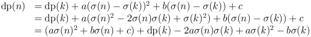
Now, let

Then, we see that  is the quantity we aim to maximize by our choice of . Adding
  (which is independent of ) to the maximum gives the correct value of
  . Also,
  is independent of , whereas
  and
and  are independent of
  , as required.
Unlike in task "acquire", we are interested in building the "upper envelope". We notice that the slope of the "maximal" line increases as increases. Since the problem statement indicates , the slope of each line is positive.
Suppose  . For
. For  we have slope
  . For
. For  we have slope
  . But
. But  ,
and since the given sequence is positive, so
,
and since the given sequence is positive, so  . We conclude that lines are added to our data structure in increasing order of slope.
Since  , query values are given in increasing order and a pointer walk suffices (it is not necessary to use binary search.)
Fully dynamic variant
The convex hull trick is easy to implement when all insertions are given before all queries (offline version) or when each new line inserted has a lower slope than any line currently in the envelope. Indeed, by using a deque, we can easily allow insertion of lines with higher slope than any other line as well. However, in some applications, we might have no guarantee of either condition holding. That is, each new line to be added may have any slope whatsoever, and the insertions may be interspersed with queries, so that sorting the lines by slope ahead of time is impossible, and scanning through an array to find the lines to be removed could take linear time per insertion
It turns out, however, that it is possible to support arbitrary insertions in amortized logarithmic time. To do this, we store the lines in an ordered dynamic set (such as C++'s std::set). Each line possesses the attributes of slope and y-intercept, the former being the key, as well as an extra  field, the minimum -coordinate at which this line is the lowest in the set. To insert a new line, we merely insert it into its correct position in the set, and then all the lines to be removed, if any, are contiguous with it. The procedure is then largely the same as for the case in which we always inserted lines of minimal slope: if the line to be added is , the line to the left is , and the line to the left of that is , then we check if the - intersection is to the left of the - intersection; if so, is discarded and we repeat; similarly, if lines
  and
and  are on the right, then can be removed if the - intersection is to the left of the - intersection, and this too is performed repeatedly until no more lines are to be discarded. We compute the new values (for , it is the - intersection, and for , it is the - intersection).
To handle queries, we keep another set, storing the same data but this time ordered by the value. When we insert or remove lines from that set (or update, in the case of above), we use the value from the element in that set to associate it with an element in this one. Whenever a query is made, therefore, all we have to do is to find the greatest value in this set that is less than the query value; the corresponding line is the optimal one .
References
- Brucker, P. (1995). Efficient algorithms for some path partitioning problems. Discrete Applied Mathematics, 62(1-3), 77-85.
- Christiano, Paul. (2007). Land acquisition. Retrieved from an archived copy of the competition problem set at http://tjsct.wikidot.com/usaco-mar08-gold
- Peng, Richard. (2008). USACO MAR08 problem 'acquire' analysis. Retrieved from http://ace.delos.com/TESTDATA/MAR08.acquire.htm
- van den Hooff, Jelle. (2010). Personal communication.
- Wang, Hanson. (2010). Personal communication.