Knuth–Morris–Pratt algorithm
The Knuth–Morris–Pratt (KMP) algorithm is a linear time solution to the single-pattern string search problem. It is based on the observation that a partial match gives useful information about whether or not the needle may partially match subsequent positions in the haystack. This is because a partial match indicates that some part of the haystack is the same as some part of the needle, so that if we have preprocessed the needle in the right way, we will be able to draw some conclusions about the contents of the haystack (because of the partial match) without having to go back and re-examine characters already matched. In particular, this means that, in a certain sense, we will want to precompute how the needle matches itself. The algorithm thus "never looks back" and makes a single pass over the haystack. Together with linear time preprocessing of the needle, this gives a linear time algorithm overall.
Contents
Motivation
The motivation behind KMP is best illustrated using a few simple examples.
Example 1
In this example, we are searching for the string  = aaa in the string
  = aaaaaaaaa (in which it occurs seven times). The naive algorithm would begin by comparing
  with
with  ,
,  with
with  , and
, and  with
with  , and thus find a match for at position 1 of . Then it would proceed to compare with , with , and with
  , and thus find a match at position 2 of , and so on, until it finds all the matches. But we can do better than this, if we preprocess and note that and are the same, and and are the same. That is, the prefix of length 2 in matches the substring of length 2 starting at position 2 in ; partially matches itself. Now, after finding that
  match
match  , respectively, we no longer care about , since we are trying to find a match at position 2 now, but we still know that
  match
match  respectively. Since we already know
 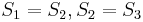 , we now know that
  match respectively; there is no need to examine and again, as the naive algorithm would do. If we now check that matches , then, after finding at position 1 in , we only need to do one more comparison (not three) to conclude that also occurs at position 2 in . So now we know that match
  , respectively, which allows us to conclude that match
  . Then we compare with
  , and find another match, and so on. Whereas the naive algorithm needs three comparisons to find each occurrence of in , our technique only needs three comparisons to find the first occurrence, and only one for each after that, and doesn't go back to examine previous characters of again. (This is how a human would probably do this search, too.)
Example 2
Now let's search for the string = aaa in the string = aabaabaaa. Again, we start out the same way as in the naive algorithm, hence, we compare with , with , and with . Here we find a mismatch between and , so does not occur at position 1 in . Now, the naive algorithm would continue by comparing with and with , and would find a mismatch; then it would compare with , and find a mismatch, and so on. But a human would notice that after the first mismatch, the possibilities of finding at positions 2 and 3 in are extinguished. This is because, as noted in Example 1, is the same as , and since  ,
,  also (so we will not find at position 2 of ). And, likewise, since
  , and , it is also true that
  , so it is pointless looking for a match at the third position of . Thus, it would make sense to start comparing again at the fourth position of (i.e., with
  , respectively). Again finding a mismatch, we use similar reasoning to rule out the fifth and sixth positions in , and begin matching again at
  (where we finally find a match.) Again, notice that the characters of were examined strictly in order.
Example 3
As a more complex example, imagine searching for the string = tartan in the string = tartaric_acid. We make the observation that the prefix of length 2 in matches the substring of length 2 in starting from position 4. Now, we start by comparing  with
with  , respectively. We find that
  does not match
  , so there is no match at position 1. At this point, we note that since and
  , and
, and  , obviously,
  and , so there cannot be a match at position 2 or position 3. Now, recall that
  and
and  , and that
  . We can translate this to
  . So we proceed to compare with . In this way, we have ruled out two possible positions, and we have restarted comparing not at the beginning of but in the middle, avoiding re-examining and .
Concept
Let the prefix of length  of string be denoted
  .
.
The examples above show that the KMP algorithm relies on noticing that certain substrings of the needle match or do not match other substrings of the needle, but it is probably not clear what the unifying organizational principle for all this match information is. Here it is:
- At each position of , find the longest proper suffix of that is also a prefix of .
We shall denote the length of this substring by  , following [1]. We can also state the definition of equivalently as the maximum
  such that
  .
.
The table  , called the prefix function, occupies linear space, and, as we shall see, can be computed in linear time. It contains all the information we need in order to execute the "smart" searching techniques described in the examples. In particular, in examples 1 and 2, we used the fact that
  , that is, the prefix aa matches the suffix aa. In example 3, we used the facts that
  . This tells us that the prefix ta matches the substring ta ending at the fifth position. In general, the table tells us, after either a successful match or a mismatch, what the next position is that we should check in the haystack. Comparison proceeds from where it was left off, never revisiting a character of the haystack after we have examined the next one.
Computation of the prefix function
To compute the prefix function, we shall first make the following observation:
- Prefix function iteration lemma[1]: The sequence
 contains exactly those values such that
  .
.
That is, we can enumerate all suffixes of that are also prefixes of by starting with , looking it up in the table , looking up the result, looking up the result, and so on, giving a strictly decreasing sequence, terminating with zero.
- Proof: We first show by induction that if appears in the sequence
 then , i.e, indeed belongs in the sequence . Suppose is the first entry in . Then
  and it is trivially true that . Now suppose is not the first entry, but is preceded by the entry
  which is valid. That is,
  . By definition,
  . But
. But  by assumption. Since
  is transitive, .
 - We now show by contradiction that if , then
 . Assume does not appear in the sequence. Clearly
  since 0 and both appear. Since is strictly decreasing, we can find exactly one
  such that
  and
and  ; that is, we can find exactly one after which "should" appear (to keep the sequence decreasing). We know from the first part of the proof that . Since the suffix of of length is a suffix of the suffix of of length , it follows that the suffix of of length matches the suffix of length of
  . But the suffix of of length also matches
  , so matches the suffix of of length . We therefore conclude that
  . But
. But  , a contradiction.
With this in mind, we can design an algorithm to compute the table . For each , we will first try to find some  such that . If we fail to do so, we will conclude that
  (clearly this is the case when
  .) Observe that if we do find such , then by removing the last character from this suffix, we obtain a suffix of
  that is also a prefix of , i.e.,
  . Therefore, we first enumerate all nonempty proper suffixes of that are also prefixes of . If we find such a suffix of length which also satisfies
  , then
  , and
, and  is a possible value of . So we will let
  and keep iterating through the sequence
  . We stop if we reach element in this sequence such that
  , and declare
  ; this always gives an optimal solution since the sequence
  is decreasing and since it contains all possible valid 's. If we exhaust the sequence, then .
Here is the pseudocode:
π[1] ← 0
for i ∈ [2..m]
    k ← π[i-1]
    while k > 0 and S[k+1] ≠ S[i]
        k ← π[k]
    if S[k+1] = S[i]
        π[i] ← 0
    else
        π[i] ← k+1
With a little bit of thought, this can be re-written as follows:
π[1] ← 0
k ← 0
for i ∈ [2..m]
    while k > 0 and S[k+1] ≠ S[i]
        k ← π[k]
    if S[k+1] = S[i]
        k ← k+1
    π[i] ← k
This algorithm takes  time to execute. To see this, notice that the value of
 k is never negative; therefore it cannot decrease more than it increases. It only increases in the line k ← k+1, which can only be executed up to  times. Therefore
 k can be decreased at most k times. But k is decreased in each iteration of the while loop, so the while loop can only run a linear number of times overall. All the other instructions in the for loop take constant time per iteration, so linear time overall.
Matching
Suppose that we have already computed the table . Here's where we apply this hard-won information. Suppose that so far we are testing position for a match, and that the first characters of have been successfully matched, that is,  . There are two possibilities: either we just continue going along and and comparing pairs of characters, or we decide we want to try out a new position in . This occurs because either
  (i.e, we've successfully located at position in , and now we want to check out other positions) or because
 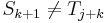 (so we can rule out the current position).
Given that 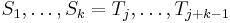 , what positions in can we rule out? Here is the result at the core of the KMP algorithm:
- Theorem: If
 then
then  is the least
  such that
  match
match  , respectively. (If
  , then
  vacuously.)
Think carefully about what this means. If does not satisfy the statement that match , then the needle does not match at position  , i.e., we can rule out the position . On the other hand, if does satisfy this statement, then might match at position , and, in fact, all the characters up to but not including
  have already been verified to match the corresponding characters in , so we can proceed by comparing
  with , and, as promised, never need to look back.
- Proof: Let
 . If
. If  , then by definition we have
  . But since
  , it is also true that
  . Therefore
  . If, on the other hand, it is not true that , then it is not true that , so it is not true that , so it is not true that . Therefore
  is a possible value of
  if and only if . Since the maximum possible value of
  is
is  , the minimum possible value of is given by
  .
.
Thus, here is the matching algorithm in pseudocode:
j ← 1
k ← 0
while j+m-1 ≤ n
    while k ≤ m and S[k+1] = T[j+k]
        k ← k+1
    if k = m
        print "Match at position " j
    if k = 0
        j ← j+1
    else
        j ← j+k-π[k]
        k ← π[k]
Thus, we scan the text one character at a time; the current character being examined is located at position  . When there is a mismatch, we use the table to look up the next possible position at which the match might occur, and try to proceed.
The fact that the algorithm scans one character at a time without looking back is more obvious when the code is cast into this equivalent form:[1]
k ← 0
for i ∈ [1..n]
    while k > 0 and S[k+1] ≠ T[i]
        k ← π[k]
    if S[k+1] = T[i]
        k ← k+1
    if k = m
        print "Match at position " i-m+1
        k ← π[k]
Here, i is identified with j+k as above. Each iteration of the inner loop in one of these two segments corresponds to an iteration of the outer loop in the other. In this second form, we can also prove that the algorithm takes  time; each time the inner while loop is executed, the value of
 k decreases, but it cannot decrease more than  times because it starts as zero, is never negative, and is increased at most once per iteration of the outer loop (i.e., at most times in total), hence the inner loop is only executed up to times. All other operations in the outer loop take constant time.
References
- ↑ 1.0 1.1 1.2 Thomas H. Cormen; Charles E. Leiserson, Ronald L. Rivest, Clifford Stein (2001). "Section 32.4: The Knuth-Morris-Pratt algorithm". Introduction to Algorithms (Second ed.). MIT Press and McGraw-Hill. pp. 923–931. ISBN 978-0-262-03293-3.