Difference between revisions of "Maximum flow"
(in progress) |
(in progress) |
||
| Line 1: | Line 1: | ||
| − | The '''maximum flow problem''' is an optimization problem in [[graph theory]]. It deals with a special kind of graph, known as a ''flow network''. A flow network is a [[directed graph]] with the following properties: | + | The '''maximum flow problem''' is an optimization problem in [[graph theory]]. It deals with a special kind of graph, known as a ''flow network''. |
| + | |||
| + | ==The flow network== | ||
| + | A flow network is a [[directed graph]] with the following properties: | ||
# There are two special nodes, the ''source'' (usually denoted ''s''), and the ''sink'' (usually denoted ''t''). | # There are two special nodes, the ''source'' (usually denoted ''s''), and the ''sink'' (usually denoted ''t''). | ||
# No edges enter the source nor leave the sink. | # No edges enter the source nor leave the sink. | ||
# To each edge we associate a non-negative real number called the ''capacity''. Thus, we can represent a flow network similarly to how we would represent a weighted graph. | # To each edge we associate a non-negative real number called the ''capacity''. Thus, we can represent a flow network similarly to how we would represent a weighted graph. | ||
| + | |||
| + | We may describe a flow network mathematically as a tuple <math>(V, E, c)</math> where <math>c:E \to [0, \infty)</math> and <math>\forall e, e \not\rightarrow s \wedge e \not\leftarrow t</math>. Here <math>c(e)</math> is the capacity of the edge <math>e</math>. <math>e \leftarrow v</math> denotes that edge <math>e</math> leaves vertex <math>v</math>, and <math>e \rightarrow v</math> denotes that edge <math>e</math> enters vertex <math>v</math>. | ||
| + | |||
A flow network may be used to model real-life systems in which some substance flows from one place (the source) to another (the sink), going through any number of intermediate locations (other nodes) along paths of various maximum capacities connecting locations (edges). This is the motivation behind the statement of the maximum flow problem. | A flow network may be used to model real-life systems in which some substance flows from one place (the source) to another (the sink), going through any number of intermediate locations (other nodes) along paths of various maximum capacities connecting locations (edges). This is the motivation behind the statement of the maximum flow problem. | ||
| − | In order to state the problem, we first have to define the concept of an ''admissible flow''. An admissible flow is an assignment of a non-negative real number to each edge (which we call the ''flow along'' that edge) such that the flow along an edge never exceeds the capacity of that edge, and such the flow "balances" at each vertex other than the source and sink, meaning that the total flow at incoming edges equals the total flow at outgoing edges at each vertex. | + | ==Admissible flows== |
| + | In order to state the problem, we first have to define the concept of an ''admissible flow''. An admissible flow is an assignment of a non-negative real number to each edge (which we call the ''flow along'' that edge), such that the flow along an edge never exceeds the capacity of that edge, and such the flow "balances" at each vertex other than the source and sink, meaning that the total flow at incoming edges equals the total flow at outgoing edges at each vertex. | ||
| + | |||
| + | Mathematically, an admissible flow is a function <math>f: E \to [0, \infty)</math> such that <math>\forall v \in V-\{s, t\}, \sum_{e \rightarrow v} f(e) = \sum_{e \leftarrow v} f(e)</math>. Here, <math>f(e)</math> is the flow along edge <math>e</math>. | ||
| + | |||
| + | Some authors, instead of requiring that <math>f(e) \geq 0</math>, use the convention that every edge <math>(u, v)</math> must have a back edge <math>(v, u)</math>, and that the flow along an edge equals the negative of the flow along the back edge. In such a case, the balance condition can be expressed as the requirement that the total incoming flow must be zero at each intermediate vertex, or, equivalently, that the total outgoing flow must be zero. Here "incoming flow" means flow along edges that enter the vertex, even if the flow along such edges is negative. | ||
| + | |||
| + | The balance condition may be thought of as a precise statement of the idea that the vertices have no capacities of their own; they serve only as connecting points for the edges and cannot store excess incoming flow nor discharge stored flow when the incoming flow is running low. | ||
| + | ===Analogies=== | ||
| + | * In one possible analogy, the edges represent pipes, each of which has some maximum rate at which it can transport water (the capacity). An admissible flow then corresponds to some way of sending water through the pipes from source to sink through a series of intermediate nodes. The rate at which water flows into an intermediate node must equal the rate at which water flows out of the same node, because the nodes can't store excess water, and water can't just come out of nowhere. | ||
| + | * In another possible analogy, the edges represent conducting wires, each of which has some maximum amount of current it can conduct before it overheats and melts; the source represents a generator and the sink represents a device that consumes electrical power. Here, the balance condition is Kirchhoff's current law, stating that the total current flowing into a vertex equals the total current flowing out of it, and corresponds to the fact that any imbalance in current would result in an accumulation of either positive or negative charge at that vertex. | ||
| + | |||
| + | ==Statement of the problem== | ||
| + | Given an admissible flow, although incoming flow and outgoing flow balance at all vertices other than the source and the sink, the same is not true at the source and sink. Indeed, we can have flow out from the source, but not in, since no edges enter the source; we can have flow into the sink but not out, since no edges leave the sink. The objective of the problem is to find an admissible flow that maximizes the total flow out of the source or into the sink. Such a flow is called a [[maximum flow]]. | ||
| + | |||
| + | '''Proposition''': The total outgoing flow at the source equals the total incoming flow at the sink. | ||
| + | |||
| + | '''Proof''': <math>\sum_{e \in E} f(e) = \sum_{v \in V} \sum_{e \rightarrow v} f(e) = \sum_{v \in V} \sum_{e \leftarrow v} f(e)</math>. These equalities are obvious because each edge enters exactly one vertex and exits exactly one vertex. Subtracting, we obtain that <math>\sum_{v \in V} \left( \sum_{e \rightarrow v} f(e) - \sum_{e \leftarrow v} f(e) \right) = 0</math>. We can break this sum down as <math>\sum_{e \leftarrow s} f(e) - \sum_{e \rightarrow t} f(e) + \sum_{v \in V-\{s, t\}} \left( \sum_{e \rightarrow v} f(e) - \sum_{e \leftarrow v} f(e) \right)</math>. The third term here is zero due to the balance condition, so we conclude <math>\sum_{e \leftarrow s} f(e) = \sum_{e \rightarrow t} f(e)</math>. We may call this quantity the total flow, <math>F</math>. This is the quantity we wish to maximize. | ||
| + | |||
| + | ==Algorithms== | ||
| + | There are a variety of algorithms for finding a maximum flow in a flow network. The simplest are the ''Ford–Fulkerson method'' and the ''preflow push algorithms''. | ||
| + | |||
| + | ===Ford–Fulkerson method=== | ||
| + | The [[Ford–Fulkerson method]] (q.v.) comprises a set of algorithms that each proceed in a series of steps, gradually building up an admissible flow until it has reached its maximum value. Each step of the algorithm takes the previous step's output, an admissible flow, as input, and produces an admissible flow of greater value, until no further refinement is possible. The input for the first step is the empty flow (<math>\forall e, f(e) = 0</math>), which is always admissible. The refinement is done by finding an ''s''-''t'' path in the flow network that can be "added" to the current admissible flow, called an ''augmenting path''. After performing this addition, the flow network has to be modified with back edges in case we wish to decrease the flow along an edge in a subsequent step of the algorithm. | ||
| + | |||
| + | There is flexibility in how to choose the augmenting path at each step. A simple approach is to always pick the path with the fewest edges; this gives the [[Edmonds–Karp algorithm]]. A faster and more sophisticated approach involves partitioning the graph into level sets by distance from the source and only considering paths in which each edge proceeds from a level to the next. This is called [[Dinic's algorithm]]. | ||
| + | |||
| + | ===Preflow push algorithms=== | ||
| + | [[Preflow push algorithms]] differ from augmenting path algorithms in that they do not maintain an admissible flow in each step, but instead maintain a ''preflow'', in which the total flow entering a vertex is allowed to ''exceed'' the total flow exiting the vertex (but not ''vice versa''). The algorithm begins by generating a preflow in which every edge leaving the source is saturated (so that the source's neighbours all have excess incoming flow). Each step of the algorithm then attempts to discharge some vertex's excess by pushing flow from that vertex to an adjacent vertex. Some flow will be discharged into the sink, and whatever flow cannot be discharged into the sink eventually finds its way back to the source. The algorithm terminates when the intermediate vertices have completely discharged all of their excess incoming flow, and thus an admissible flow has been found. | ||
| + | |||
| + | ===Other approaches=== | ||
| + | The max flow problem may be expressed as a [[linear program]] and solved using the techniques of linear programming. Here the vector to be optimized corresponds to the flow <math>f</math>, and has one entry for each edge in the graph. Both the capacity constraints and the balance condition are linear, and may be expressed in the form <math>A\mathbf{x} \leq \mathbf{b}</math>. The value of the flow is also a linear function of the vector <math>\mathbf{x}</math>. Details are left as an exercise for the reader. | ||
| − | + | Even more sophisticated approaches were given by King, Rao, and Tarjan (1994) and Orlin (2012). Combining the two approaches gives a lower bound of <math>O(VE)</math> on the general max flow problem, the best known to date. | |
Revision as of 20:57, 7 September 2013
The maximum flow problem is an optimization problem in graph theory. It deals with a special kind of graph, known as a flow network.
Contents
The flow network
A flow network is a directed graph with the following properties:
- There are two special nodes, the source (usually denoted s), and the sink (usually denoted t).
- No edges enter the source nor leave the sink.
- To each edge we associate a non-negative real number called the capacity. Thus, we can represent a flow network similarly to how we would represent a weighted graph.
We may describe a flow network mathematically as a tuple  where
where  and
and  . Here
  is the capacity of the edge
  .
.  denotes that edge leaves vertex
  , and
, and  denotes that edge enters vertex .
A flow network may be used to model real-life systems in which some substance flows from one place (the source) to another (the sink), going through any number of intermediate locations (other nodes) along paths of various maximum capacities connecting locations (edges). This is the motivation behind the statement of the maximum flow problem.
Admissible flows
In order to state the problem, we first have to define the concept of an admissible flow. An admissible flow is an assignment of a non-negative real number to each edge (which we call the flow along that edge), such that the flow along an edge never exceeds the capacity of that edge, and such the flow "balances" at each vertex other than the source and sink, meaning that the total flow at incoming edges equals the total flow at outgoing edges at each vertex.
Mathematically, an admissible flow is a function  such that
  . Here,
  is the flow along edge .
Some authors, instead of requiring that  , use the convention that every edge
  must have a back edge
  , and that the flow along an edge equals the negative of the flow along the back edge. In such a case, the balance condition can be expressed as the requirement that the total incoming flow must be zero at each intermediate vertex, or, equivalently, that the total outgoing flow must be zero. Here "incoming flow" means flow along edges that enter the vertex, even if the flow along such edges is negative.
The balance condition may be thought of as a precise statement of the idea that the vertices have no capacities of their own; they serve only as connecting points for the edges and cannot store excess incoming flow nor discharge stored flow when the incoming flow is running low.
Analogies
- In one possible analogy, the edges represent pipes, each of which has some maximum rate at which it can transport water (the capacity). An admissible flow then corresponds to some way of sending water through the pipes from source to sink through a series of intermediate nodes. The rate at which water flows into an intermediate node must equal the rate at which water flows out of the same node, because the nodes can't store excess water, and water can't just come out of nowhere.
- In another possible analogy, the edges represent conducting wires, each of which has some maximum amount of current it can conduct before it overheats and melts; the source represents a generator and the sink represents a device that consumes electrical power. Here, the balance condition is Kirchhoff's current law, stating that the total current flowing into a vertex equals the total current flowing out of it, and corresponds to the fact that any imbalance in current would result in an accumulation of either positive or negative charge at that vertex.
Statement of the problem
Given an admissible flow, although incoming flow and outgoing flow balance at all vertices other than the source and the sink, the same is not true at the source and sink. Indeed, we can have flow out from the source, but not in, since no edges enter the source; we can have flow into the sink but not out, since no edges leave the sink. The objective of the problem is to find an admissible flow that maximizes the total flow out of the source or into the sink. Such a flow is called a maximum flow.
Proposition: The total outgoing flow at the source equals the total incoming flow at the sink.
Proof: 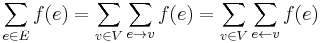 . These equalities are obvious because each edge enters exactly one vertex and exits exactly one vertex. Subtracting, we obtain that
 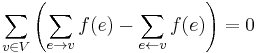 . We can break this sum down as
 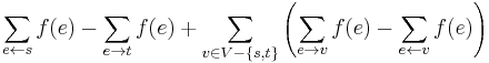 . The third term here is zero due to the balance condition, so we conclude
 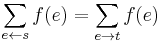 . We may call this quantity the total flow,
  . This is the quantity we wish to maximize.
Algorithms
There are a variety of algorithms for finding a maximum flow in a flow network. The simplest are the Ford–Fulkerson method and the preflow push algorithms.
Ford–Fulkerson method
The Ford–Fulkerson method (q.v.) comprises a set of algorithms that each proceed in a series of steps, gradually building up an admissible flow until it has reached its maximum value. Each step of the algorithm takes the previous step's output, an admissible flow, as input, and produces an admissible flow of greater value, until no further refinement is possible. The input for the first step is the empty flow ( ), which is always admissible. The refinement is done by finding an s-t path in the flow network that can be "added" to the current admissible flow, called an augmenting path. After performing this addition, the flow network has to be modified with back edges in case we wish to decrease the flow along an edge in a subsequent step of the algorithm.
There is flexibility in how to choose the augmenting path at each step. A simple approach is to always pick the path with the fewest edges; this gives the Edmonds–Karp algorithm. A faster and more sophisticated approach involves partitioning the graph into level sets by distance from the source and only considering paths in which each edge proceeds from a level to the next. This is called Dinic's algorithm.
Preflow push algorithms
Preflow push algorithms differ from augmenting path algorithms in that they do not maintain an admissible flow in each step, but instead maintain a preflow, in which the total flow entering a vertex is allowed to exceed the total flow exiting the vertex (but not vice versa). The algorithm begins by generating a preflow in which every edge leaving the source is saturated (so that the source's neighbours all have excess incoming flow). Each step of the algorithm then attempts to discharge some vertex's excess by pushing flow from that vertex to an adjacent vertex. Some flow will be discharged into the sink, and whatever flow cannot be discharged into the sink eventually finds its way back to the source. The algorithm terminates when the intermediate vertices have completely discharged all of their excess incoming flow, and thus an admissible flow has been found.
Other approaches
The max flow problem may be expressed as a linear program and solved using the techniques of linear programming. Here the vector to be optimized corresponds to the flow  , and has one entry for each edge in the graph. Both the capacity constraints and the balance condition are linear, and may be expressed in the form
  . The value of the flow is also a linear function of the vector
  . Details are left as an exercise for the reader.
Even more sophisticated approaches were given by King, Rao, and Tarjan (1994) and Orlin (2012). Combining the two approaches gives a lower bound of  on the general max flow problem, the best known to date.