Prefix sum array and difference array
Given an array of numbers, we can construct a new array by replacing each element by the difference between itself and the previous element, except for the first element, which we simply ignore. This is called the difference array, because it contains the first differences of the original array. We will denote the difference array of array  by
by  . For example, the difference array of
 ![A = [9, 2, 6, 3, 1, 5, 0, 7]](/wiki/images/math/7/f/9/7f9d88c652b184dc4db1a19714f6dd80.png) is
is ![D(A) = [2-9, 6-2, 3-6, 1-3, 5-1, 0-5, 7-0]](/wiki/images/math/e/3/5/e35ce6a5ac5351ad3daf63f72445d05b.png) , or
, or ![[-7, 4, -3, -2, 4, -5, 7]](/wiki/images/math/a/d/d/add580769fa99a870317b923383072b7.png) .
.
We see that the difference array can be computed in linear time from the original array, and is shorter than the original array by one element. Here are implementations in C and Haskell. (Note that the Haskell implementation actually takes a list, not an array, and will work fine for infinite lists.)
// D must have enough space for n-1 ints
void difference_array(int* A, int n, int* D)
{
    for (int i = 0; i < n-1; i++)
        D[i] = A[i+1] - A[i];
}
d :: [Int] -> [Int] -- NB: The general type signature should be (Num a) => [a] -> [a]
d a = zipWith (-) (tail a) a
The prefix sum array is the opposite of the difference array. Given an array of numbers and an arbitrary constant  , we first append onto the front of the array, and then replace each element with the sum of itself and all the elements preceding it. For example, if we start with , and choose to append the arbitrary value
  to the front, we obtain
 ![P(-8, A) = [-8, -8+9, -8+9+2, -8+9+2+6, ..., -8+9+2+6+3+1+5+0+7]](/wiki/images/math/3/0/a/30a6494f688a01d72adad9f368016095.png) , or
, or ![[-8, 1, 3, 9, 12, 13, 18, 18, 25]](/wiki/images/math/5/c/c/5cc1dad3f6d3c0ccea7d7d3dd92c5bc8.png) . Computing the prefix sum array can be done in linear time as well, and the prefix sum array is longer than the original array by one element:
. Computing the prefix sum array can be done in linear time as well, and the prefix sum array is longer than the original array by one element:
// P must have enough space for n+1 ints
void prefix_sum_array(int c, int* A, int n, int* P)
{
    P[0] = c;
    for (int i = 0; i < n; i++)
        P[i+1] = P[i] + A[i];
}
p :: Int -> [Int] -> [Int] -- NB: The general type signature should be (Num a) => a -> [a] -> [a]
p = scanl (+)              -- NB: This is the same as p c a = scanl (+) c a
Note that every array has an infinite number of possible prefix sum arrays, since we can choose whatever value we want for . For convenience, we usually choose  . However, changing the value of has only the effect of shifting all the elements of
  by a constant. For example,
 ![P(15, A) = [15, 24, 26, 32, 35, 36, 41, 41, 48]](/wiki/images/math/2/f/5/2f55d6c3a47d61dae3b77320f34e8d9d.png) . However, each element of
. However, each element of  is exactly 23 more than the corresponding element from
  .
.
The functions  and
and  carry out reverse processes. Given an nonempty zero-indexed array :
-
 for any . For example, taking the difference array of
 ![P(-8, A) = [-8, 1, 3, 9, 12, 13, 18, 18, 25]](/wiki/images/math/0/2/b/02b6898dffbc07ad061a917cb0a015c4.png) gives
gives ![[9, 2, 6, 3, 1, 5, 0, 7]](/wiki/images/math/a/3/e/a3e4109270a19cac82c7e91bec7564e4.png) , that is, it restores the original array .
, that is, it restores the original array . -
 . Thus, taking
 ![D(A) = [-7, 4, -3, -2, 4, -5, 7]](/wiki/images/math/f/4/4/f4480db6ad3c47e96c7874fcfcea1336.png) and
and  (initial element of ), we have
 ![P(A_0, D(A)) = [9, 2, 6, 3, 1, 5, 0, 7]](/wiki/images/math/9/7/a/97a41ef3e4d9b2e3dde402ac06122ea8.png) , again restoring the original array .
, again restoring the original array .
Analogy with calculus
These two processes—computing the difference array, and computing a prefix sum array—are the discrete equivalents of differentiation and integration in calculus, which operate on continuous domains. An entry in an array is like the value of a function at a particular point.
- Reverse processes:
- for any . Likewise
 for any .
 - . Likewise
 .
.
-
- Uniqueness:
- A differentiable function
 can only have one derivative,
  . An array can only have one difference array, .
 - A continuous function has an infinite number of antiderivatives,
 , where can be any number in its domain, but they differ only by a constant (their graphs are vertical translations of each other). An array has an infinite number of prefix arrays , but they differ only by a constant (at each entry).
- A differentiable function
- Given some function
![f:[a,b]\to\mathbb{R}](/wiki/images/math/3/3/2/332d0f0f6103ad3c4ec22d3af5b36e7c.png) , and the fact that
, and the fact that  , an antiderivative of
  , satisfies
  , we can uniquely reconstruct . That is, even though has an infinite number of antiderivatives, we can pin it down to one once we are given the value the antiderivative is supposed to attain on the left edge of 's domain. Likewise, given some array and the fact that , a prefix sum array of , satisfies
  , we can uniquely reconstruct .
 - Effect on length:
- is shorter than by one element. Differentiating gives a function
 (shortens the closed interval to an open interval).
 - is longer than by one element. Integrating
 gives a function
 ![F:[a,b] \to \mathbb{R}](/wiki/images/math/1/9/b/19b17cac5b2437be7e4aa88212b6ddc4.png) (lengthens the open interval to a closed interval).
(lengthens the open interval to a closed interval).
-
Because of these similarities, we will speak simply of differentiating and integrating arrays. An array can be differentiated multiple times, but eventually it will shrink to length 0. An array can be integrated any number of times.
Use of prefix sum array
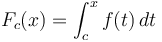
The Fundamental Theorem of Calculus also has an analogue, which is why the prefix sum array is so useful. To compute an integral  , which is like a continuous kind of sum of an infinite number of function values
  , we take any antiderivative , and compute
  . Likewise, to compute the sum of values
  , we will take any prefix array and compute
  . Notice that just as we can use any antiderivative because the constant cancels out, we can use any prefix sum array because the initial value cancels out. (Note our use of the left half-open interval.)
Proof:  and
and  . Subtracting gives
 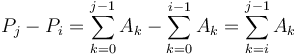 as desired.
This is best illustrated via example. Let as before. Take ![P(0,A) = [0, 9, 11, 17, 20, 21, 26, 26, 33]](/wiki/images/math/c/4/7/c473217b3594e5fed86c3fbef7cc3894.png) . Then, suppose we want
. Then, suppose we want  . We can compute this by taking
  . This is because
  .
.
Example: Counting Subsequences (SPOJ)
Computing the prefix sum array is rarely the most difficult part of a problem. Instead, the prefix sum array is kept on hand because the algorithm to solve the problem makes frequent reference to range sums.
We will consider the problem Counting Subsequences from IPSC 2006. Here we are given an array of integers  and asked to find the number of contiguous subsequences of the array that sum to 47.
To solve this, we will first transform array into its prefix sum array  . Notice that the sum of each contiguous subsequence
  corresponds to the difference of two elements of , that is, . So what we want to find is the number of pairs
  with
with  and
and  . (Note that if
  , we will instead get a subsequence with sum -47.)
However, this is quite easy to do. We sweep through from left to right, keeping a map of all elements of we've seen so far, along with their frequencies; and for each element  we count the number of times
  has appeared so far, by looking up that value in our map; this tells us how many contiguous subsequences ending at
  have sum 47. And finally, adding the number of contiguous subsequences with sum 47 ending at each entry of gives the total number of such subsequences in the array. Total time taken is
  , if we use a hash table implementation of the map.