Difference between revisions of "Heavy-light decomposition"

Revision as of 03:19, 25 September 2013 (edit) 192.190.204.201 (Talk) ← Older edit		Revision as of 09:38, 10 November 2013 (edit) (undo) 188.61.185.123 (Talk) (Undo addition which screwed up the entire structure of the page) Newer edit →
Line 1:		Line 1:
−	Heavy-light decomposition
−
−	Heavy-light decomposition - it is a common method which allows to solve many problems, which reduce to queries from a tree.
−
−	The simplest example of this type of problems - is the next task. Given a tree, each node is assigned a number. There have been queries of the form (a, b), where a and b - number of vertices of the tree, and you want to know the maximum number of vertices in the path between a and b.
−
−	Description of the algorithm
−
−	So, suppose we are given a tree G with n vertices, suspended for a certain root.
−
−	The point of this decomposition is to split a tree in several ways so that for any vertex v turned out that if we are to rise from v to the root, then we change the path of no more than \ log n paths. In addition, all paths should not cross each other in the ribs.
−
−	Clearly, if we learn to seek a decomposition for any tree, it will bring any kind of inquiry "to learn something on the way from a to b" to several requests like "learn something on the interval [l; r] k-th the way. "
−
−	Construction of heavy-light decomposition
−
−	Count for each vertex v the size of its subtree s (v) (ie, the number of vertices in the subtree of vertex v, including the very top).
−
−	Next, we consider all edges leading to the sons of a vertex v. We call an edge (v, c) severe, if it leads to a vertex c such that:
−
−	s (c) \ ge \ frac {s (v)} {2} ~ ~ ~ ~ \ Leftrightarrow [...]
−
−	All other edges are said to light. Obviously, one of v may come down heavy at most one edge (since otherwise a vertex v had two sons would be the size s (v) / 2, taking into account the very top of v gives a size of 2 \ cdot s ( v) / 2 + 1> s (v), ie a contradiction).
−
−	Now we construct a decomposition tree itself into disjoint paths. Consider all the vertices of which does not go down no hard edges, and we will go from each of them up until you get to the root of the tree or not to go through a slight edge. As a result, we obtain a number of ways - we will show that this is the desired way heavy-light decomposition.
−
−	The proof of the correctness of the algorithm
−
−	First, note that the resulting algorithm will be non-intersecting paths. In fact, if any two paths have a common edge, it would mean that some of the top comes down two heavy edges, which can not be.
−
−	Second, we show that down from the root to any vertex, we will change the path of no more than \ log n paths. In fact, the passage down the slight edge reduces the size of the current subtree more than doubled
−
−	s (c) <\ frac {s (v)} {2} ~ ~ ~ ~ \ Leftrightarrow ~ ~ [...]
−
−	Thus, we could not pass over \ log n light edges. However, the move from one track to another, we can only through a slight edge (because every path, except ending at the root, has a slight edge in the end, and get right in the middle of the way, we can not).
−
−	Consequently, the path from the root to any vertex, we can not change over \ log n paths as required.
−
−	Applications in solving problems
−
−	In solving problems it is sometimes convenient to consider the heavy-light as a set of vertex-disjoint paths (not edge-disjoint). It's enough of each path, delete the last edge, if it is an easy point-blank - if no properties are not violated, but now each vertex belongs to exactly one path.
−
−	Below we consider some typical problems that can be solved using the heavy-light decomposition.
−
−	Pay special attention to the problem of the sum of the numbers on the road, because this is an example of the problem, which can be solved by simpler techniques.
−	The maximum number in the path between two vertices
−
−	Given a tree, each node is assigned a number. There have been queries of the form (a, b), where a and b - number of vertices of the tree, and you want to know the maximum number of vertices in the path between a and b.
−
−	We construct a pre-heavy-light decomposition. Above each of the resulting construct the tree through the segments to the maximum, which will search for the top with the maximum number ascribed in this segment of the path for the O (\ log n). Although the number of paths in the decomposition of heavy-light can reach n-1, the total size of all paths is the value of O (n), so the total size of the trees and the segments will be linear.
−
−	Now, in order to respond to a query (a, b) find the lowest common ancestor of l vertices (for example, by lifting binary). Now the problem is reduced to two inquiries: (a, l) and (b, l), each of which we can answer this way: we find, in what way is the lower top, make a request to this path, we go into the top-end of the way, again to determine in which way we were and make a request to him, and so on, until we reach the path that contains l.
−
−	Carefully should be the case when, for example, a and l are in one way - then the maximum request to this path should be done not on the suffix, as in the domestic subsegments.
−
−	Thus, in answer to a subquery, we go through the O (\ log n) paths, each of them making a request to the maximum suffix or prefix / subsegments (request for prefix / subsegments could be only one time).
−
−	So we got a solution for the O (\ log ^ 2 n) on a request.
−
−	If you have additional predposchitat highs in every way for all suffixes, we get a solution for the O (n \ log n) - as request the maximum suffix not happen only once, when we get to the top of l.
−
−	The sum of the numbers on the path between two vertices
−
−	Given a tree, each node is assigned a number. There have been queries of the form (a, b), where a and b - number of vertices of the tree, and you want to know the sum of the path between vertices a and b. The variant of this problem when there are additional requests for changes in the number, assigned a particular node.
−
−	Although this problem can be solved with the help of heavy-light decomposition, by building on each tree for the sum of the segments (or just predposchitav partial sums, if there are no requests for changes in the task), this problem can be solved by simpler techniques.
−
−	If the modification requests are not available, the amount of learning on the path between two vertices can be parallel to the LCA with the search algorithm, two vertices in the binary lifting - just during pre-LCA to calculate not only the 2 ^ k-th ancestor of each vertex, but the amount of numbers on the way to this ancestor.
−
−	There is also a fundamentally different approach to this problem - to consider the Eulerian traversal of the tree and construct a tree of segments on it. This algorithm is discussed in the article with a similar solution of the problem. (And if there are no requests for modifications - it is enough to do predposchetom partial sums, without a tree of segments.)
−
−	Both of these methods give relatively simple solutions with the asymptotics O (\ log n) per query.
−
−	Repainting edges of the path between two vertices
−
−	Given a tree, each edge originally painted white. There have been queries of the form (a, b, c), where a and b - number of vertices, c - the color, which means that all the edges on the path from a to b should be repainted in the color c. Require repainting after all to tell, but in the end turned the edges of each color.
−
−	The solution - just do a painting of a tree of segments on a segment on a set of ways of heavy-light decomposition.
−
−	Each request is repainted on the road (a, b) turn into two sub-query (a, l) and (b, l), where l - the lowest common ancestor of vertices a and b (found, for example, lifting a binary algorithm), and each of these subqueries - in O (\ log n) queries to the trees above the track segments.
−
−	Altogether it is a solution with the asymptotic behavior O (\ log ^ 2 n) on a request.
−
−	Problems in the online judges
−
−	The list of tasks that can be solved using the heavy-light decomposition:
−
−	* TIMUS # 1553 "Caves and Tunnels" [difficulty: medium]
−
−	* IPSC 2009 L "Let there be rainbows!" [Difficulty: medium]
−
−	* SPOJ # 2798 "Query on a tree again!" [Difficulty: medium]
−
−	* Codeforces Beta Round # 88 E "A tree or a tree" [difficulty: high]
−
	The '''heavy-light''' (H-L) '''decomposition''' of a rooted tree is a method of partitioning of the vertices of the tree into disjoint paths (all vertices have degree two, except the endpoints of a path, with degree one) that gives important asymptotic time bounds for certain problems involving trees. It appears to have been introduced in passing in Sleator and Tarjan's analysis of the performance of the [[link-cut tree]] data structure.		The '''heavy-light''' (H-L) '''decomposition''' of a rooted tree is a method of partitioning of the vertices of the tree into disjoint paths (all vertices have degree two, except the endpoints of a path, with degree one) that gives important asymptotic time bounds for certain problems involving trees. It appears to have been introduced in passing in Sleator and Tarjan's analysis of the performance of the [[link-cut tree]] data structure.

---

Revision as of 09:38, 10 November 2013

The heavy-light (H-L) decomposition of a rooted tree is a method of partitioning of the vertices of the tree into disjoint paths (all vertices have degree two, except the endpoints of a path, with degree one) that gives important asymptotic time bounds for certain problems involving trees. It appears to have been introduced in passing in Sleator and Tarjan's analysis of the performance of the link-cut tree data structure.

Definition

The heavy-light decomposition of a tree is a coloring of the tree's edges. Each edge is either heavy or light. To determine which, consider the edge's two endpoints: one is closer to the root, and one is further away. If the size of the subtree rooted at the latter is more than half that of the subtree rooted at the former, the edge is heavy. Otherwise, it is light.

Properties

Denote the size of a subtree rooted at vertex as .

Suppose that a vertex has two children and and the edges - and - are both heavy. Then, 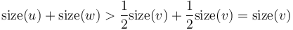. This is a contradiction, since we know that . (, of course, may have more than two children.) We conclude that there may be at most one heavy edge of all the edges joining any given vertex to its children.

At most two edges incident upon a given vertex may then be heavy: the one joining it to its parent, and at most one joining it to a child. Consider the subgraph of the tree in which all light edges are removed. Then, all resulting connected components are paths (although some contain only one vertex and no edges at all) and two neighboring vertices' heights differ by one. We conclude that the heavy edges, along with the vertices upon which they are incident, partition the tree into disjoint paths, each of which is part of some path from the root to a leaf.

Suppose a tree contains vertices. If we follow a light edge from the root, the subtree rooted at the resulting vertex has size at most ; if we repeat this, we reach a vertex with subtree size at most , and so on. It follows that the number of light edges on any path from root to leaf is at most .

Applications

The utility of the H-L decomposition lies in that problems involving paths between nodes can often be solved more efficiently by "skipping over" heavy paths rather than considering each edge in the path individually. This is because long paths in trees that are very poorly balanced tend to consist mostly of heavy edges.

To "skip" from any node in the tree to the root:

while current_node ≠ root
     if color(current_node,parent(current_node)) = light
          current_node = parent(current_node)
     else
          current_node = skip(current_node)

In the above, color(u,v) represents the color (heavy or light) of the edge from u to v, parent(v) represents the parent of a node v, and skip(v) represents the parent of the highest (i.e., least deep) node that is located on the same heavy path as node v. (It is so named because it allows us to "skip" through heavy paths.) In order for the latter to be implemented efficiently, every node whose parent link is heavy must be augmented with a pointer to the result of the skip function, but that is trivial to achieve.

What is the running time of this fragment of code? There are most a logarithmic number of light edges on the path, each of which takes constant time to traverse. There are also at most a logarithmic number of heavy subpaths, since between each pair of adjacent heavy paths lies a light path. We spend at most a constant amount of time on each of these, so overall this "skipping" operation runs in logarithmic time.

This might not seem like much, but let's see how it can be used to solve a simple problem.

Lowest common ancestor

The H-L decomposition gives an efficient solution to the lowest common ancestor (LCA) problem. Consider first a naive solution:

function LCA(u,v)
     while depth(u) < depth(v) and u ≠ v
          v = parent(v)
     while depth(u) > depth(v) and u ≠ v
          u = parent(u)
     while u ≠ v
          u = parent(u)
          v = parent(v)
     return u

(In this code, u and v are the nodes whose LCA is desired.)

This solution can take time proportional to the height of the tree, which can be up to linear. However, we can use the "skip" operation of the H-L decomposition to do much better:

function LCA_improved(u,v)
     let last = root
     while u ≠ v
          if depth(u) > depth(v)
               swap(u,v)
          if color(v,parent(v)) = light
               last = root
               v = parent(v)
          else
               last = v
               v = skip(v)
     if last = root
          return u
     else
          return last

Here's how this code works: in each iteration of the while loop, the deeper of the two nodes is advanced up the tree (that is, if its parent link is light, it becomes its parent, otherwise it "skips", as previously described). Note that if the two nodes are equally deep, one of them still gets advanced; this is intentional and it does not matter which one is advanced. When the two nodes become equal, we are done.

Or are we? Suppose that the highest edges on the paths from each node to the LCA are light. Then, it is clear that the while loop ends with both nodes now pointing to the LCA, after having advanced through the respective light edges. If, however, one is heavy, there is a possibility that we "overshoot"; that is, that we end up at a node higher in the tree than the actual LCA. If this occurs, then the last advancement before its occurrence is from the actual LCA to the ending node (convince yourself of this by drawing a diagram if necessary), so that all we have to do is "remember" the last node visited in this case. That is what the last variable holds. (If both final links to the LCA are light, it is set to the root of the tree, which is otherwise impossible, to indicate this.) Notice that we do not have to consider the case in which both final links to the LCA are heavy, since this is impossible; two child links from a node cannot both be heavy, so these two heavy links would have to be the same link, making the child of that link a lower common ancestor (a contradiction).

Dynamic distance query

Now consider the following problem: A weighted, rooted tree is given followed by a large number of queries and modifications interspersed with each other. A query asks for the distance between a given pair of nodes and a modification changes the weight of a specified edge to a new (specified) value. How can the queries and modifications be performed efficiently?

First of all, we notice that the distance between nodes and is given by . We already know how to efficiently solve lowest common ancestor queries, so if we can efficiently solve queries of a node's distance from the root, a solution to this problem follows trivially.

To solve this simpler problem of querying the distance from the root to a given node, we augment our walk procedure as follows: when following a light edge, simply add its distance to a running total; when following a heavy path, add all the distances along the edges traversed to the running total (as well as the distance along the light edge at the top, if any). The latter can be performed efficiently, along with modifications, if each heavy path is augmented with a data structure such as a segment tree or binary indexed tree (in which the individual array elements correspond to the weights of the edges of the heavy path).

This gives time for queries, since it consists of two "skips" and a LCA query, all of which take logarithmic time or better. It might seem that we have to ascend logarithmically many heavy paths each of which takes logarithmic time, but this is not the case; only the first one, if we start out on it, has to take logarithmic time to query; for the others, which we skip over in their entirety, we can just look up a variable indicating the sum of all weights on that path, which can be updated in constant time when any edge on that path is updated. An update, merely an update to the underlying array structure, takes time also.

References

• Wang, Hanson. (2009). Personal communication.
• D. D. Sleator and R. E. Tarjan, A data structure for dynamic trees, in "Proc. Thirteenth Annual ACM Symp. on Theory of Computing," pp. 114–122, 1981.